Procedutal Velocity Field Creation

Applicable to Stoke MX 2 and higher, Last Edited on June 5, 2014

Overview

The following tutorial discusses the creation of custom Velocity Fields using the Field Magma object introduced in Stoke MX 2.

In this tutorial, we will create a simple sine wave in 3D space and advect Particle Flow particles using the Stoke Field Follow operator, but the same setup could be used to drive a Stoke Particle Simulation.

The Base Scene

• Start a new 3ds Max scene.
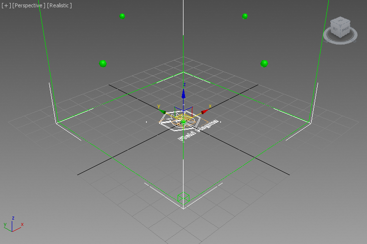
• Hold down the SHIFT key and select “Create a Field Magma object…” from the Stoke menu - this will create a default grid with size of 100 along all axes, centered at the World Origin.
• In the Modify panel, click the button “Base To Icon” to move the grid 50 units up and place the base of the grid in the XY plane of the world coordinate system. Note that moving the Field Magma icon does NOT affect the position of the grid - it is always defined in world space coordinates!
• In the Viewport Display, change the Display drop-down list from Large Dots to Velocity.
• Enter 0.03 in the value next to the Norm.Length checkbox (which should remain unchecked).
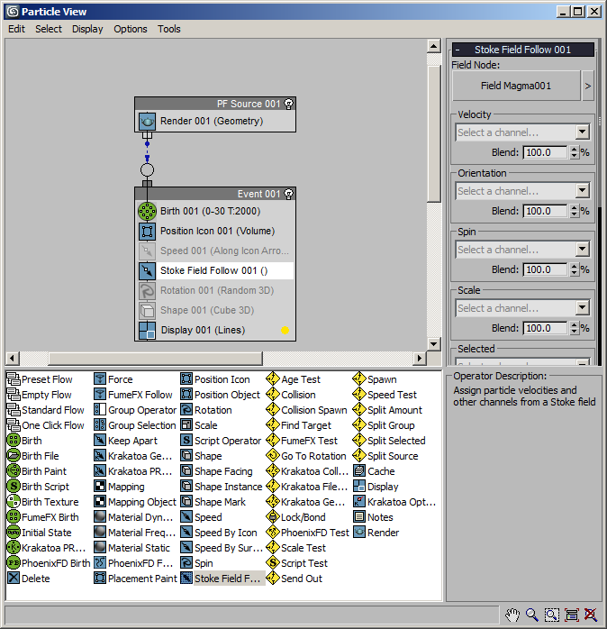
• Select 3ds Max Menus > Graph Editors > Particle View to open the Particle Flow Editor.
• Drag a Standard Flow into the view - this will create a default system at the world origin.
• Disable the Speed, Rotation and Shape operator for now.
• Switch the Display operator to Lines and set its color to yellow.
• Select the the Birth operator and increase the particle count to 2000.
• Select the PF Source 001 node and change the Viewport % to 100.0 and the Viewport Integration Step to Half Frame to produce smooth motion.
• Drag a Stoke Field Follow from the depot and insert it between the disabled Speed and Rotation operators.
• Pick the Field Magma001 object as the Field Node of the Stoke Field Follow operator.

RESULT: We are now ready to set up our Magma flow to generate a Velocity Field.

Setting Up a Simple 2D Sine Wave Velocity Field

Next, we will set up the Velocity Field which will drive the Particle Flow particles.

• Select the Field Magma001 object in the scene and click the Open Magma Editor button.
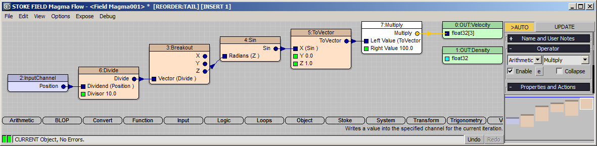
• Select the existing Velocity Output node and press SHIFT+P to connect a Position InputChannel node.
• Press CTRL+R to switch to Auto-Reorder mode.
• Click the “Extract Z” button in the command panel of the Magma Editor to insert a Breakout node between the InputChannel and the Output nodes - the Velocity Output will turn red because the output is a Float, but a Vector is expected. Ignore this error for now as we will fix it in a few steps.
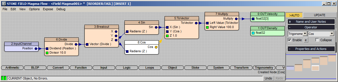
• With the Breakout node still selected, press the [ key to insert a Sin operator (or alternatively press R and then I).
• With the Sin operator selected, click C for Convert category, then V for ToVector. This will pipe the result of the Sin operator into the X input socket of the ToVector operator, producing a changing value from 0.0 through 1.0, 0.0, -1.0 and again 0.0 as the Z axis of the position changes between 0.0 and 2*Pi.
• Enter 1.0 for the Z component of the ToVector to add a vertical motion to the Velocity Field.
• Select the InputChannel Position node and click / on the Numeric Keypad to insert a Divide operator, and enter 10.0 for the Divisor.
• Select the ToVector operator and press the * key on the Numeric Keypad to insert a Multiply operator, then enter 100.0 for the Right Value. NOTE that this value is a rather arbitrary scaler and can be changed to produce faster or slower motion as needed.

RESULT: Moving the time slider shows that the Particle Flow particles are now moving according to the Sine Wave we created in the Field Magma object, esp. when looking through the Front viewport (since we are setting only the X and Z axes of the field vectors).

Limited Vs. Infinite Fields

You will notice that when the particles leave the top of the grid, they stop being affected by the Velocity Field. This is because the default settings of the Field Magma object include a “Limit Field To Bounds” checkbox which is on by default. As result, the field is only defined inside the bounding box of the object!

• Uncheck the “Limit Field To Bounds” checkbox and play back again.

RESULT: Moving the time slider now shows the particles following the sine wave even outside of the Grid.

NOTE that some grid-based operators in Magma as well as some Stoke Field Modifiers like Stoke Field Fluid Motion only operate within the bounding box defined by the base object, and won’t produce valid data outside of it. The unlimited calculation outside of the Grid Bounds is only possible when all operators within the flow as well as all modifiers on the stack are not dependent on Grid calculations.

Similarly, the Spacing value will affect grid-based operations and produce more or less precise values as it controls the grid voxel size. But when the flow is fully procedural, the Spacing will only affect the viewport display. If the display is turned off, the flow will be evaluated only for the points requested by the Particle Flow via the Stoke Field Follow operator. Increasing the particle count will also increase the number of evaluations of the flow.

Going 3D

Now let’s modify our flow a bit to add a motion along the Y axis too.

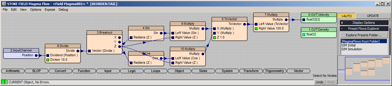
• Click the Z output socket of the Breakout operator and connect to the Y input socket of the ToVector operator.
• Click to select the newly created connection and press the ] key to insert a Cos operator.
• Change the Spacing value of the Grid to 5.0 to draw less samples - as mentioned above, when the flow is fully procedural like the current one, the Velocity Field can be calculated at ANY point in 3D space, and the Spacing only controls the display samples.

RESULT: Looking in the perspective viewport, the particles are now following a helix in space, moving like the cork screw.

Increasing The Radius Over Distance

By multiplying the X and Y components of the Velocity by the Z distance from the XY plane, we can increase the radius of our Helix as the particles move away from the origin.

• Select the Sin operator and press the * key on the Numeric keypad to insert a Multiply operator.
• Select the Cos operator and press again the * key.
• Drag a connection from the Z output socket of the Breakout operator to the Right Values of both Multiply operators.

RESULT: Playing back the animation now shows that the helix is getting wider and wider with height.

Controlling The Radius Bias

Currently the radius is increasing linearly with the increase of the height of the helix. We can easily control the bias by inserting a Power operator.

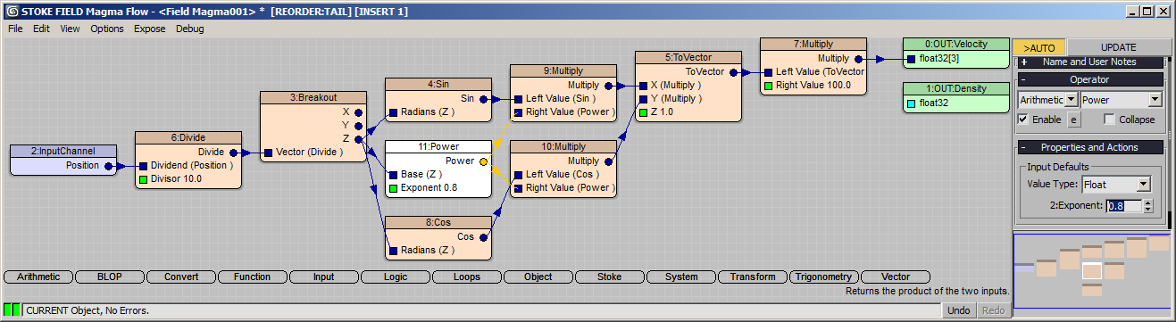
• Select the connection going from the Z output of the Breakout to the Multiply operator behind the Sin node and press the 6 key on the top row of the keyboard (the one with the ^ character) - a Power operator will be inserted.
• Connect the output of the Power operator to the Right Value socket of the Multiply operator behind the Cos node.
• Change the Exponent value of the Power operator to a value less than 1.0 to reduce the speed with which the radius is increasing as the Position Z increases. A value of about 0.8 should be good for now.

RESULT: The Helix’ Radius grows slower now.

Blending Stoke Field Follow’s Influence With Existing Speed

The Stoke Field Follow operator provides a Blend value which controls how much of the Velocity coming from the Field object should be mixed with the existing Speed from the previous integration step. By default, a Blend value of 100.0 fully overwrites any existing speed in the particles.

• Open the Particle View and select the Stoke Field Follow operator.
• Change the Blend value under the Velocity group from 100.0% to 10%
• Enable the Speed operator above the Stoke Field Follow operator.
• Select the Speed operator and change its Direction drop-down list from the default “Along Icon Arrow” to “Random Horizontal”.

RESULT: Initially, the particles will have their random horizontal motion, with 10% of the Helical Wave motion added on each step. Over time, most of the random horizontal motion will be lost as more and more of the Velocity Field is added, resulting in a randomized initial motion that changes the overall shape of the cloud as it continues to move within the field.

What Is Next?

In the next tutorial, we will use the same spiral Velocity Field to drive the motion of a FumeFX Simulation!