Simple Plume Simulation

Applicable to Stoke MX 2

Overview

The Stoke Field Simulator lets you create both simple and rather complex fluid simulation setups.

In the following example, we will use a mesh volume to emit into a Scalar field and advect it by a Velocity field dependent on the Scalar field. This will let us simulate both the temperature rising up and the buoyancy of smoke particles, producing a swirling plume of smoke. The Basic Scene ============================================= * Create a Geosphere with Radius 20.0 at the World Origin (it could be anywhere else, but it would require the moving of the Grid to that location, so World Origin is simpler). * Hold down the SHIFT key and select the Create a Field SIMULATOR Object… entry from the Stoke menu. * Change the Grid Z Min. to -30.0 and Z Max. to 200.0.

Rising Density

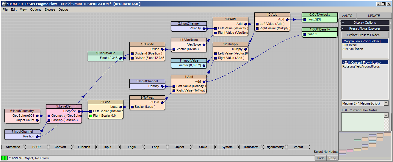
• Press the Open SIMULATION Flow… button.
• Select the existing Velocity output node and press SHIFT+V to connect a new Velocity InputChannel node.
• Select the existing Density output node and press SHIFT+D to connect a new Density InputChannel node.
• Press the + key on the Numeric Keypad to insert an Add operator into the existing flow between the Density input and output.
• Drag with the mouse from the second socket of the Add node and release to show the node menu. Pick the LevelSet operator from the Stoke category. This operator takes a mesh and turns it into a grid the same way PRT Volume or Stoke Particle Simulator turn meshes into grids to seed particles in them. The LevelSet exposes a Distance channel which will have negative values inside the volume.
• Drag from the first socket of the LevelSet operator and release to create a GeometryInput node.
• Pick the GeoSphere as the mesh to convert to a LevelSet.
• Drag from the second socket of the LevelSet operator and release to create an InputChannel Position node.
• Select the LevelSet node and press L for Logic and S for Less to insert a Less operator behind the LevelSet. The default of the second socket is 0.0 which is exactly what we want - output 1 when the sample point is inside the mesh (Distance field is negative), or 0 when it is outside.
• In the Less operator, click the Convert To Float button. This will insert a ToFloat behind the Less, turning the boolean values intoo 1.0 and 0.0.
• Select the Velocity InputChannel node and press Numpad + to insert another Add operator.
• Hold SHIFT and then press 3 on the top row of the keyboard to connect an InputVector with value of [0,0,1] (up!).
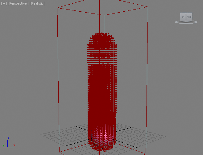
• Press the SIMULATE button in the 3ds Max command panel.
• Once the simulation is done, change the Viewport Display settings to Mask: Density

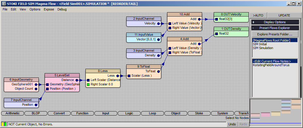
RESULT: On each simulation step, we inject a Density value of 1.0 to the existing Density field inside the GeoSphere, and Velocity of 0,0,1 in every voxel of the Grid.

Playing back the simulation in the viewport will show just a column of Density values rising up, as we requested via the above Magma flow.

Adjusting The Velocity By Density

We are pumping values into the two fields simulation on every step. If we assume that the inside of the GeoSphere is burning and the Density channel represents both the Temperature AND the Smoke of our simulation, we can easily cause the Velocity to be higher where the Temperature is higher!

• Select the InputValue [0,0,1] node and press the Numpad * key to insert a Multiply node.
• Connect with the mouse from the output of the Add node that is connected directly to the Density output to the second socket of the new Multiply node.
• Switch the Viewport Display to Display: Velocity.
• Set the Norm.Length value to 0.1 while leaving the checkbox unchecked.
• Press SIMULATE again and wait for the simulation to finish.

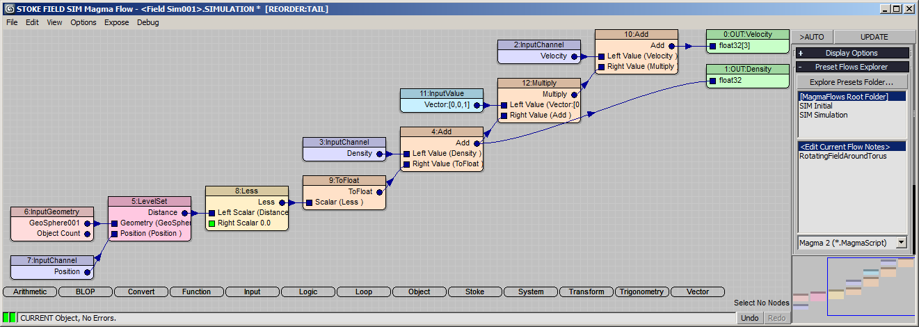
RESULT: We are now setting the Velocity to zero where the Density/Temperature is 0.0, and to higher and higher values where the Density/Temperature is rising.

Because the default Solver is set to Simple Fluid Solver - see the drop-down list at the bottom of the Simulation rollout in the 3ds Max Command Panel - the removal of the Divergence will produce swirling Velocities due to the variation in Velocity values in space.

Advecting Stoke Particles

To really appreciate the Velocity Field we just created, let’s advect some Stoke particles to visualize it.

• Select both the GeoSphere and the Stoke Field Sim objects and pick Create a STOKE Particle Reflow Simulator… option from the Stoke menu, then click in the viewport to place the icon. The two objects will be added to the respective lists automatically!
• Change the Rate/Frame to 1000.
• Select the GeoSphere on the Distribution Sources list and switch from Surface to Volume.
• Enter 3.331 as Volume Spacing (this the Grid Size of the Field Sim).
• Check the TextureCoord channel to be acquired at birth.
• Press the SIMULATE button and wait for the particles to be advected.
• In the Viewport Display rollout, switch Color to TextureCoord and Display to Velocity.

RESULT: The particles are emitted in the volume of the GeoSphere and form a mushroom cloud before existing the Simulation Grid.

Adjusting The Speed

Since the Velocity and Density are now connected, we can produce faster or slower motion by either changing the up vector added to the Velocity field before the multiplication by Density, or multiply the result of the LevelSet Boolean To Float conversion before it is used to inject more Density and modulate the value added to the Velocity.

Let’s do the former.

• Change the InputValue from [0,0,1] to [0,0,0.2] to reduce the buoyancy value 5 times.

Adding Turbulence

In addition to the up vector added to the Velocity to represent the “heat” rising, we can introduce a Noise field to cause some irregularities.

• Select the InputChannel Velocity node and press Numpad + to insert another Add node.
• Drag from the second socket of the new Add node and release, then select Function > VecNoise.
• Uncheck the VecNoise >Normalize option.
• Drag from the Vector input socket of the VecNoise and connect to the existing Position node.
• Select the new wire and press the Numpad / key to insert a new Divide node.
• Press Ctrl+1 to connect an InputValue Float value, then change to 12.345 - this controls the Scale of the Noise.
• Press SIMULATE button of the Field Sim again.
• Once done, press the SIMULATE button in the Stoke Particle Simulator.

RESULT: The Velocity field now contains a static random component, producing a more distorted simulation. Due to the reduction of the up vector, the plume rises slower too.

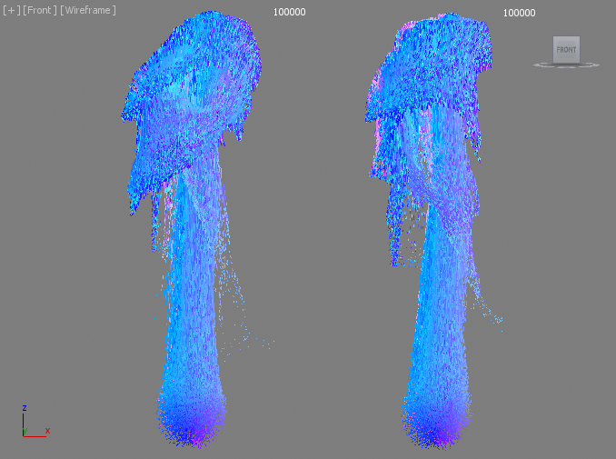
Rendering In Krakatoa

Below is the result of simulating with Rate of 100,000 particles for up to 10,000,000 particles on frame 100, rendered in Krakatoa MX 2.3 using Particle mode. Density 1.0E-3, 4 Passes Motion Blur, lit by one Spot Light:

Here is the same rendered as Voxels with Size 1.0:

Animating The Velocity Field Vector Noise

In the previous simulation, we used a static Noise Vector Field to produce random motion in the particles. In some cases, we might want the Noise Field to be animated too. While it does not make a huge difference in this case where the Velocity due to rising heat is significant, in other cases it might be useful, so here is how to implement it in the Magma flow:

• Select the connection between the Position InputChannel and the Divide operator before the VecNoise node.
• Press the Numpad + key to insert a new Add operator.
• Press SHIFT+0 to connect a Vector InputValue. Enter [0.1,0.1,-0.1] as value.
• Press the Numpad * key to insert a new Multiply operator.
• Press the `/~ key or CTRL+SPACEBAR to open the ActiveType and type in Frame, then hit ENTER - this will connect a new InputScript operator with Script “CurrentTime.frame as float” to the Multiply operator.

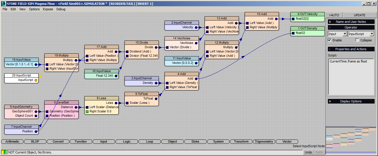
RESULT: If we would simulate again (as a new version), the VecNoise field will be moving 1 unit along X, Y and Z every 10 frames, thus producing a different result when simulating the Stoke particles.

We could also keyframe the Vector InputValue to the desired offsets, but this would require changes whenever the time range of the scene changes, while the above approach is procedural as it depends on the current frame which always advances when time changes. To increase or decrease the motion or invert the direction along an axis, just adjust the InputValue Vector components.

Volumetric Rendering

The Density field generated in this tutorial can also be rendered directly as voxels without advecting any particles.

You can use either the Stoke Atmospheric Effect with a supporting renderer like Default Scanline or V-Ray, or export the field to FXD file sequence and render using FumeFX in case you own that plugin.

The animation below shows the Density field of the Stoke Field Sim above saved to an FXD file sequence and rendered using FumeFX in the Default Scanline renderer:

Next

In the next tutorial, we will use this Field Simulation data to affect a geometry object using the Genome procedural modifier and its InputField Magma operator.