Wetmap Field Simulation

Applicable to Stoke MX 2, Last Edited March 3, 2016

Overview

The following tutorial discusses the creation of Wetmaps from particle data using the Field Simulation object introduced in Stoke MX 2.

A Wetmap stores history information about the contact of a surface with a fluid. In our example, we will use a simple Particle Flow system and a Collision with a mesh object. We will record information about the proximity of particles to the surface and produce a field which, when converted to a texture map, will control the surface look by blending a Dry and a Wet material.

The Base Scene

In our test, we will use a very simple setup:

• Create a Plane primitive at the origin with size of 120.0 x 120.0 units.
• Rotate the Plane at 30 degrees about X.
• Create a Standard Particle Flow and move up 60.0 units along the +Z.
• Change the PFlow to emit 1000 particles over 30 frames and display 100% in the viewport
• Set the Integration step to be the same for viewport and rendering.
• Create a default Gravity SpaceWarp and apply to the PFlow via a Force operator.
• Create a default Drag SpaceWarp and apply to the PFlow using the same Force operator.
• Create a UCollision Deflector SpaceWarp using the rotated Plane, apply after the Force using a Collision test.
• Set the UCollision to Bounce 0.1, Variations 0.0%, Chaos 15.0%, Friction 55.0%, Inherit Vel. 1.0.
• Set the Shape operator to Sphere 20-sides with Size of 5.0.
• Set the Display operator to Geometry.

Creating The Stoke Field Simulator

Select the Plane and select the 3ds Max Menu bar > Stoke > Create a Field SIMULATOR object… item - the Stoke Field Simulator will be created with the size of the Plane’s World Bounding Box. Set the Spacing to 2.0 units.

Setting Up The Initial Flow

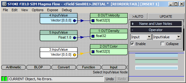
• Click Open INITIAL Flow
• Select the existing Velocity Output and press SHIFT+0 to connect an InputValue Vector of [0,0,0].
• Select the existing Density Output and press CTRL+1 to connect an InputValue Float of 1.0.
• Press SHIFT+CTRL+C to create a new Color Output channel and press SHIFT+0 to connect it to an InputValue Vector of [0,0,0].
• Close the INITIAL Flow.

Setting Up The Simulation Flow

• Click Open SIMULATION Flow.
• Select the Velocity output and press SHIFT+V to connect to an InputChannel Velocity.
• Select the Density output and press SHIFT+D to connect to an InputChannel Density.
• Press SHIFT+CTRL+C to create a Color Output.
• Press SHIFT+C to connect to a Color InputChannel.
• Press the + key on the Numpad to insert an Add operator.
• With the Add node still selected, press O for Object and then S for ParticleSumRadius.
• Drag from the Particles input socket and release over empty area to create an InputParticles node.
• Pick the Particle Flow and select Event 001. NOTE: The Event picker dialog might lose focus after the viewport click due to a glitch in 3ds Max - simply perform Alt+Tab to another application and then back to 3ds Max, and the dialog should regain focus. Alternatively, use the H key to use the Select By Name dialog to pick the Particle Flow instead of clicking in the viewport!
• Drag from the Lookup Point socket and release over an empty area to create a Position InputChannel.
• Select the ParticleSumRadius and press Ctrl+3 to connect an InputValue with 3.0 to the Radius input socket.
• Select the wire connecting the NumParticles output socket of the ParticleSumRadius and the Add operator behind the Color InputChannel and press L for Logic and G fro Greater.
• Change the type of the second socket in the Greater operator to Integer and leave as 0 value.
• Select the wire coming out of the Greater operator and press the ? key to insert a Switch.
• With the Switch node selected, press CTRL+W and then SHIFT+CTRL+W to swap the first two and the last two sockets and bring the connection to the 3rd Boolean socket.
• With the Switch node selected, press SHIFT+0 twice to connect two InputValue Vectors to its two sockets.
• Enter [0.1,0.1,0.1] into the first InputValue node, and [-0.05,-0.05,-0.05] into the second InputValue.
• Select the wire coming out of the Add operator and click B for BLOP, V for Vector category and E for ClampVector.
• With the ClampVector BLOP selected, press SHIFT+0 twice to connect two InputValue Vectors of [0,0,0] to the two sockets.
• Enter [2,2,2] into the second InputValue Vector.

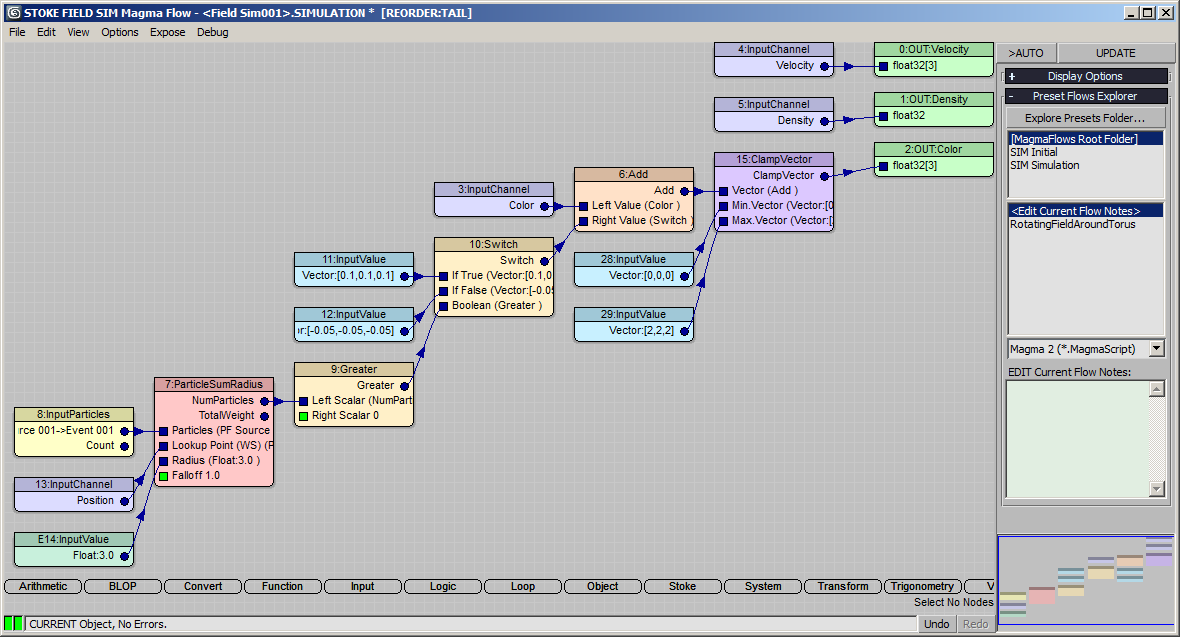
RESULT: If we would simulate now, when a particle is found within 3.0 units of a grid voxel, the color in that voxel will be incremented by 0.1. If there is no particle found, the value will be decremented by 0.05. The resulting Color value’s components will be clamped between 0.0 and 2.0, so no voxel can go below 0.0 (dry), and the maximum “wetness” value would be 2.0 (where 1.0 is already white). This way, if a voxel is in contact with particles for 20 or more frames, it will reach maximum wetness, and it would take 40 frames of no contact with particles before that voxels becomes dry again.

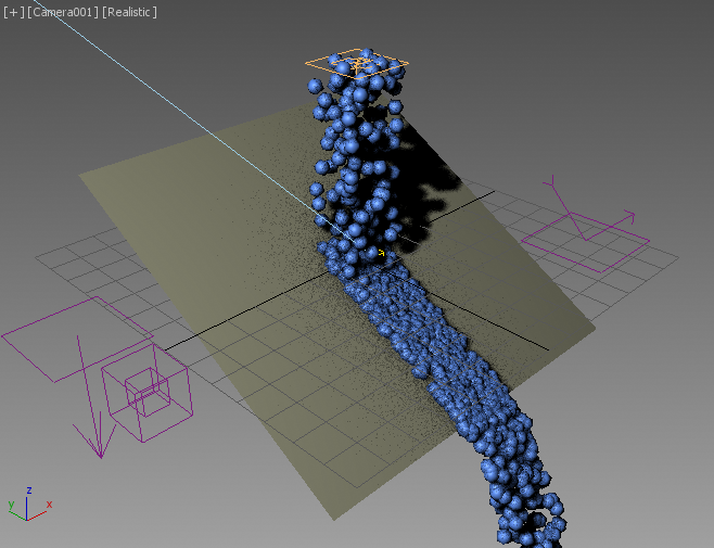
• Press the SIMULATE button and wait for the processing to finish.
• Change the Display settings to show the Color channel as Color and you should see a back&white grid of sample points representing the wetness information as you move the time slider.

Passing The Wetness Field To A Material

We can now convert this Field data into a texture map. But first we need to create a Field Loader to break some Circular Dependencies… Our Field Simulation depends on the PFlow Particle. PFlow depends on the Collision which depends on the Deflector which in turn depends on the Plane. Thus, we cannot directly assing a Stoke Field Texmap to the Plane and pick the Stoke Field Simulator because this would cause a circular dependency. Since all data is already cached to disk as VDB files, all we need is a Field Loader.

Alternatively, baking the Particle Flow to a PRT sequence using Krakatoa and using a PRT Loader as the input would also break the Circular Dependency.

• Click the [+] icon next to the >Use Disk Cache button in the Field Sim object - this will create a Field Loader with the current cache as input sequence.
• Let’s first visualize the field as a texture map without blending two materials.
• Open the 3ds Max Compact Material Editor.
• Select the Plane and assign the first Standard material to it.
• Click the Diffuse map slot and pick a Field Texmap.
• Pick the Field Loader from the scene as the Field Source and select Color as the source channel.

RESULT: At this point, you can render the Plane using the Default Scanline or any other mesh renderer - a black & white map will appear at the contact spots where the particles are sliding over the surface of the Plane.

NOTE: The Field Texmap cannot be displayed in the viewports.

Blending Two Materials Using The Wetmap

• In the 3ds Max Material Editor, create a new Blend Material.
• Open the first material and add a Noise to the Bump map slot. Set Noise to Fractal with Size 5.0.
• Go up one level and drag to Copy the top material into the second slot.
• Go to the second material and change its settings to make it look wet. For example, increase its Specularity, reduce its Opacity (making a wet paper become more transparent, for example), etc.
• Copy the Field Texture created in the previous step into the Mask socket to control the mixing using its Black & White values.
• Optionally, set up better lighting, set up a Camera with MPass Motion Blur, create some geometry behind the plane to reveal via the opacity/transparency changes in the material and so on…
• Optionally, if you have Thinkbox Frost, you could mesh the Particle Flow using Zhu/Bridson mode instead of rendering the actual spherical particles, or use BlobMesh to produce a similar result…

RESULT: If you would render the sequence now, the two materials defined in the Blend material will be mixed according to the Field Texmap, producing a wet look behind the particle trail that dries out as the particles move on.

Controlling The Contact History

We can contol how fast the surface becomes wet and how quickly it becomes dry again by tweaking the two InputValue Vectors going into the Switch operator.

Setting the second InputValue to [0,0,0] will cause the surface to stay “wet” forever. This could be useful if you want to paint a surface to a different color using particles - setting the decrement value to [0,0,0] will leave a color splat that will never fade off.

If you want the Field Texmap to only reach a shade of gray and never become white, you can adjust the VectorClamp BLOP’s Max. value.

Note that you can also collect non-grayscale values, or use the Red, Green abd Blue channels to store different types of information about the contacts.