Krakatoa, RealFlow and Frost
Overview
The following tutorial discusses the use of Krakatoa and Frost to load, process, mesh and render particle data generated by Next Limit’s RealFlow fluid simulation software.
The tutorial describes the workflow in Krakatoa MX 2, but the approach is applicable to Krakatoa 1.6.x. The differences between the two releases will be pointed out where necessary.
While this demo was created using RealFlow 5, the same principles apply to RealFlow 2012 and higher.
The RealFlow Test Simulation For this tutorial, we will use a very simple setup consisting of a Hybrido simulation.
A Sphere emitter produces a stream of particles which splash around in a box-shaped volume.
Loading RealFlow BIN Files in 3ds Max
Let’s load the BIN file sequence generated by RealFlow using a Krakatoa PRT Loader.
Note that even though there is an option to save Krakatoa PRT files out of RealFlow 2012, we will use the native BIN file sequence. On the one hand, this will allow users of RealFlow 5 to use this tutorial, on the other hand, the PRT Loader performs some coordinate system conversions when loading BIN files that are more difficult to perform when loading PRT files saved from RealFlow 2012.
- Create a PRT Loader by holding the SHIFT key and selecting “Create a PRT Loader…” option in the Krakatoa Menu. Alternatively, hold SHIFT and click the PRT icon if you have created a Krakatoa toolbar as instructed in the Krakatoa documentation.
- Add the BIN file sequence saved by the RealFlow simulation to the PRT Loader’s file list.
- Click the “% of Render” button in the Viewport rollout and select 100.0 from the list - this will set the PRT Loader to display all particles.
- Drag the time slider to see the particles moving. Go to the last frame of the simulation (in the case of the demo scene used in this example, this was frame 200).
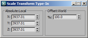
- You will notice that the size of the particle cloud is very small when compared to the home grid or the PRT Loader’s icon. This is because most simulation packages including RealFlow use metric units (SI) of meter, kilogram and second to perform their calculations. As result, one generic unit in this case represents a whole meter, and the bounding box of the particle cloud is just a few units in total.
Assuming that the 3ds Max System Settings default to 1 Generic Unit = 1 inch, we have to scale up the PRT Loader 39.3701 times (3937.01 percent) because 1 meter has 100 cm, and one inch contains 2.54 cm. Thus, 100.0/2.54=39.3701:
Color By Velocity Using Magma
In the RealFlow viewports, the Color of the particles is typically defined by their Velocity - slow particles are shaded in darker blue, fast particles are shaded in white. This provides a very useful representation of the particle Velocity and allows the user to determine how the particles are moving.
There are several ways to produce a similar effect in the 3ds Max viewports using a Magma modifier.
Note that the following examples are from Krakatoa MX 2 using the Magma 2 system which has several features that are not supported in Krakatoa 1.6.1 and earlier. The basic workflows are the same though.
- Select the PRT Loader.
- Add a Magma modifier to the stack using the “Add Krakatoa Channels Modifier (KCM)…” option from the Krakatoa Menu, the KCM icon in the toolbar (if available), or by selecting the “MagmaModifier” entry from the 3ds Max Modifiers list. Note that the name “Krakatoa Channels Modifier” is used interchangeably with “Magma”.
- Open the MagmaFlow Editor.
- Press Ctrl+O to create a new Output node. (In Krakatoa 1.6.1’ MagmaFlow Editor, the Output node already exists)
- Set the Output channel to “Color” (In 1.6.1, it will default to “Color”)
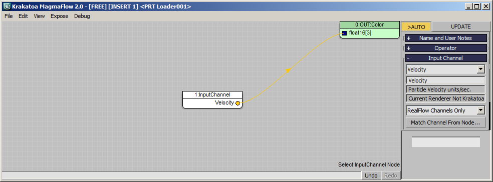
- Press SHIFT+V to create an InputChannel node set to “Velocity”.
RESULT: If you drag the time slider, you will see bright colors in the viewport representing the actual velocities stored by RealFlow in the BIN file.
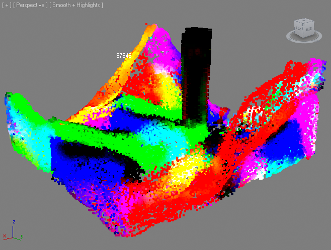
Note that areas with dark colors might have velocity components with negative sign. For example the pouring stream has X and Y mostly 0 and Z is negative. Since we are not really interested in this type of colorization, we won’t deal with removing the sign at this point.
Blending Two Colors Using Velocity Magnitude
A much better way to display the Velocity as Color is to blend two colors, for example blue and white, based on the Magnitude of the Velocity value normalized between 0.0 and 1.0. The Magnitude is the Length of the Vector and other than the Velocity Vector itself has only one component, in other words it is a Float.
- Starting with the previous Velocity->Color flow, select the Velocity input and press the V key for Vector, then M for Magnitude - a new Magnitude node will be inserted between the two existing nodes.
- Press Ctrl+R to switch to Reorder mode - the flow will be reordered automatically anbd the word [REORDER] will appear in the title bar. Adding new nodes will automatically rearrange the flow.
- We now want to “normalize” the Velocity in the range from 0 to 15 (this is an arbitrary range based on the simulation at hand, a higher or lower values might be needed depending on the data). The value of 15 would be Velocity at which the particles turn completely white. To do this, select the Magnitude node and press the / key (Divide) on the Numeric Keypad and enter 15 in the Default value of the second socket. (in v1.6.1, you will have to connect a Float Input with a value of 15 to provide the Divisor).
- With the Divide operator selected, press F for Function and then B for Blend to create a Blend operator. The Divide operator will be connected to the first input socket, but we want it to be connected to the third. Press Ctrl+W to swap the first and the second sockets, then SHIFT+Ctrl+W to swap the second and the third.
- We now want to wire a blue color into the first socket and white into the second. With the Blend node still selected, press SHIFT+3 and SHIFT+7 to create two InputValue nodes with these colors.
- In the View menu of MagmaFlow 2.0, select the “Show COLOR SWATCHES in InputValue nodes” option - the colors selected in the two inputs will appear in the nodes.
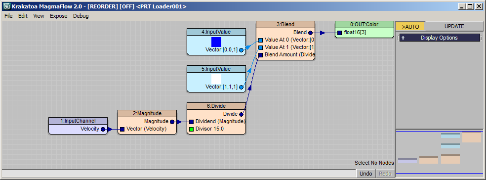
RESULT: At this point, dragging the time slider will display the particles with colors in the range from blue to white depending on their Velocity Magnitude.
Implementing Minimum and Maximum Ranges
The RealFlow Velocity as Color display provides both a Min. and a Max. value for the Velocity Range, while in the above example we assumed a Minimum of 0.0. It is very easy to implement both.
- Select the Magnitude node and press the - key (Subtract) in the Numeric Keypad. Alternatively, press A for Arithmetic and T for subTract.
- With the Subtract node selected, press Ctrl+5 to create a Float InputValue with a value of 5.0. Rename it to “Min.”
- Click and drag from the second socket of the Divide operator and release in the empty background of the editor. Select Arithmetic / Subtract from the menu.
- Drag from the output of the Min. Input node to the second socket of the new Subtract operator.
- Drag from the first input socket of the new Subtract operator and release over the empty background of the editor. Select Input / InputValue:Float from the menu.
- Rename the new InputValue to “Max.” and change its value to 15.0.
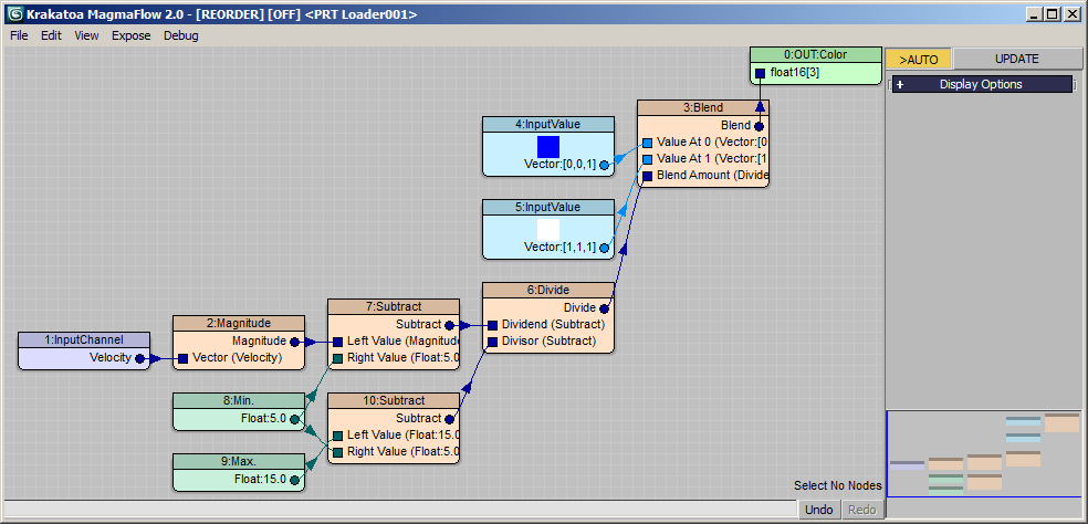
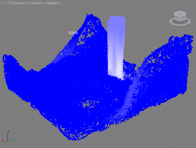
RESULT: The particles with Velocity Magnitude between 0.0 and 5.0 are now displayed as dark blue, the ones with Magnitude in the range from 5.0 to 15.0 will be shaded as a gradient from blue to white, faster particles would still be white.
Mapping A Gradient Ramp By Velocity Magnitude
An alternative approach to colorizing the particles based on their Velocity would involve the use of a Gradient Ramp texture map controller by a Mapping channel generated in the Magma modifier.
- Disable the existing Magma modifier.
- Add a new empty Magma modifier to the PRT Loader.
- Press Ctrl+O to create an Output node, set it to Channel “Mapping2”
- Press Ctrl+V to create a Velocity input node.
- Press V and M to create a Magnitude operator.
- Press / to insert a Divide operator, enter 15 in the second socket’s default.
- Press C and then V to insert a Convert > ToVector operator. We only care about the U component (which is the X of the ToVector), but connecting the Divide to all 3 inputs would also be ok.
- Open the 3ds Max Compact Material Editor.
- Assign the first default Standard material to the PRT Loader.
- Assign a Gradient Ramp texture map to its Diffuse Map slot.
- Set the Gradient Ramp to Mapping Channel 2 (same as in the Output of the Magma Modifier!)
- Uncheck the U Tiling to clamp the Mapping to the range from 0 to 1
- Set the colors in the Ramp from blue to white (or any way you want them)
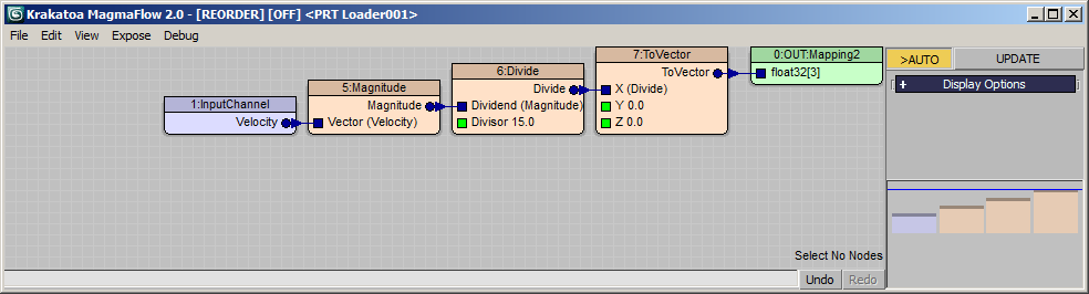
RESULT: If you move the time slider now, the colors of the particles will be based on the Magnitude of the Velocity mapped onto the Gradient Ramp’s colors.
Creating a Frost Mesh From the PRT Loader
In the next step, we will create a blob mesh from the RealFlow particles using Thinkbox’ FROST Particle Mesher.
- Select the PRT Loader.
- Click the FROST icon in the Frost Toolbar (if customized), or create a Frost object using the Create tab and pick the PRT Loader as the Source
- Hide the PRT Loader
- Set the Radius to 4.0 units and the Meshing mode Zhu/Bridson.
- Set the Viewport and Render Meshing Quality to Relative, 1.0
- Set the Zhu/Bridson Blend Radius to 2.5
- Set the Velocity To Map Channel to 3 (we will need this later)
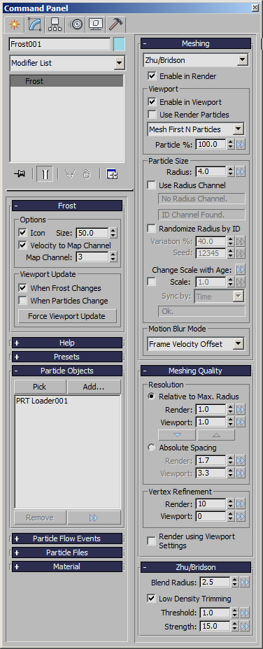
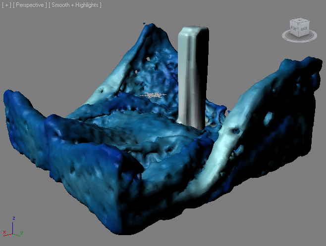
RESULT: The Frost mesh will appear in the viewport in its own object (wireframe) color.
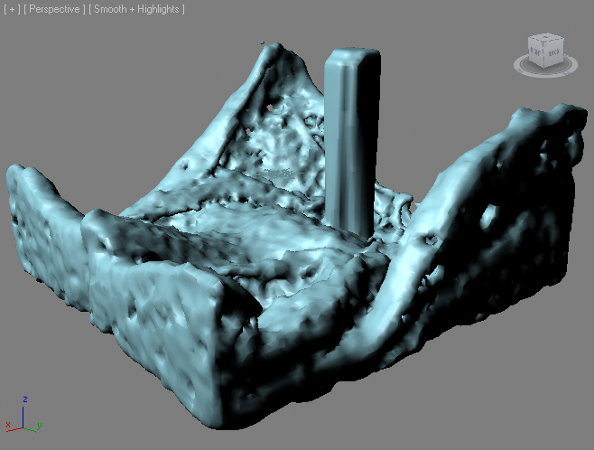
Displaying The Particle Color On The Frost Mesh
The PRT Loader particles had a Color channel defined by a Gradient Ramp using Mapping generated from the Velocity Magnitude. Displaying this color on the mesh in the viewport is very easy:
- Select the FROST object, right-click in the viewport and select Object Properties from the QuadMenu.
- In the Object Properties dialog, check “Vertex Channel Display” and press the “Shaded” checkbutton.
- Press OK to exit.
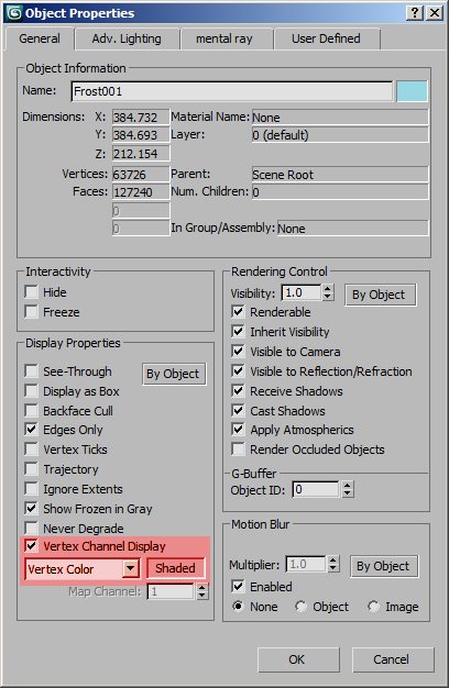
RESULT: The FROST Mesh will now show the Colors acquired from the source particles as Vertex Colors in the viewport.
Note that you will need to assign a Material with a Vertex Color Map in the Diffuse Map slot to make the colors visible in a geometry renderer like Default Scanline, mental ray, V-Ray, finalRender or Brazil r/s.
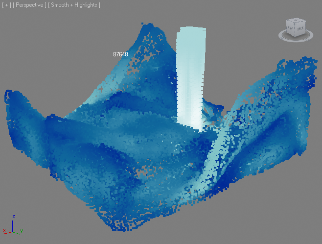
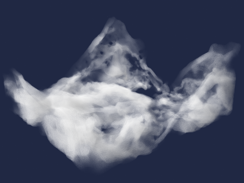
Increasing the Particle Count using PRT Volume
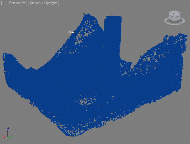
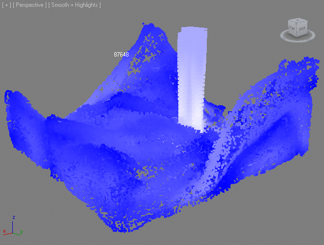
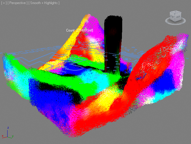
In the simulation at hand, the particle count reaches only around 80K on the last frame 200. While this is enough to produce a usable FROST mesh, it is not nearly enough to render as particles (points) in Krakatoa - the image below shows a Krakatoa particle rendering on frame 200:
As already demonstrated in another tutorial, Krakatoa and Frost can be used to produce a denser cloud of particles by filling the Frost mesh using a Krakatoa PRT Volume object and copying the Velocities via a Mapping channel.
- Select the FROST object and select the “Create PRT Volume…” option in the Krakatoa menu, or optionally press the VOL icon in the Krakatoa toolbar (if available).
- Set the “Viewport Spacing” property to 3.0
- Set the “Spacing” property controlling the render-time spacing to 2.0.
- Enable the Subdivide Region and leave it at Subdivisions: 1.
- Add a Magma modifier and open the MagmaFlow Editor.
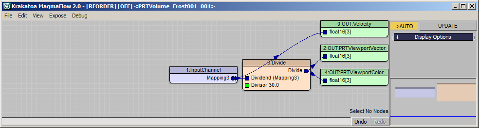
- Press Ctrl+O to create an Output node and set it to Velocity channel.
- Drag from the Output’s input socket and release in the empty background, select Input / InputChannel.
- Set the Input Channel to Mapping3 - this is the channel we saved the Velocities to when we created the FROST object!
- Let’s visualize the Velocity in the viewport as both Vectors and Colors.
- Press Ctrl+O two times and set the second Output node to PRTViewportVector and the third to PRTViewportColor.
- Note that this last step cannot be performed directly in Krakatoa 1.6.x, because MagmaFlow does not support multiple output nodes in that version. To achieve the same result, you will have to add multiple Krakatoa Channels Modifiers to the modifier stack and output the Velocity individually to each Output channel.
- Deselect all nodes.
- Press / to create a Divide operator. Enter 30 in the second socket’s default value. Wire the Input Channel into its first socket, and the output of the Divide to the second and third Output ndoes. We had to do this because the value in the Velocity channel is in Generic Units Per Second, but we want to display it Per Frame. Assuming the Frame Rate is 30 fps, we have to divide by 30 to scale the Velocities down for display purposes.
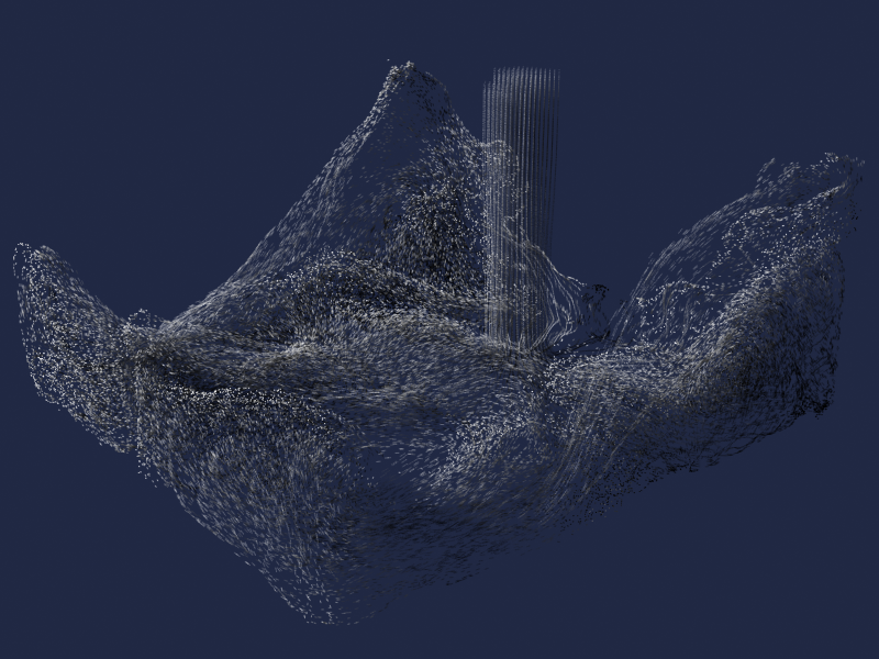
RESULT: The Velocity will now be copied from the Mapping3 channel of the FROST mesh into the PRT Volume’s particles, and the data will be visualized as colorful lines in the viewports. You will notice that these are the same colors we saw in the beginning of the tutorial, just shown as lines. As you can see, the velocities of the original 87K particles survived the trip through the FROST mesh and now live on in the PRT Volume’s particles!
Rendering Using Krakatoa Particles
At this point, the PRT Volume should provide enough particles to render as a point cloud.
- Create a Spot Light to illuminate the particles.
- Assign a White Standard Material to the PRT Volume object.
- Enable Krakatoa as the current renderer using the Krakatoa menu.
- Set the Final Pass Density to 5.0/-2
- Enable the Lighting Pass Density and set it to 1.0/-2
- Enable Motion Blur, check Jittered Motion Blur and set Particle Segments to 8.
- Enable Iterative mode and render at resolution of 800x600
RESULT: The 7.6 million particles look like a milky foam - these are 100 times more particles than in the original RealFlow simulation.

Isolating Foam By Velocity
We saw previously how we can change the Color of the particles based on the Velocity Magnitude. We can apply the same principle to the particles’ Density to isolate some particles and make them visible to the renderer, while making all others invisible by setting their Density to 0. We won’t apply this to all fast-moving particles, only to a small range of velocities that appear plausible when looking at the final result.
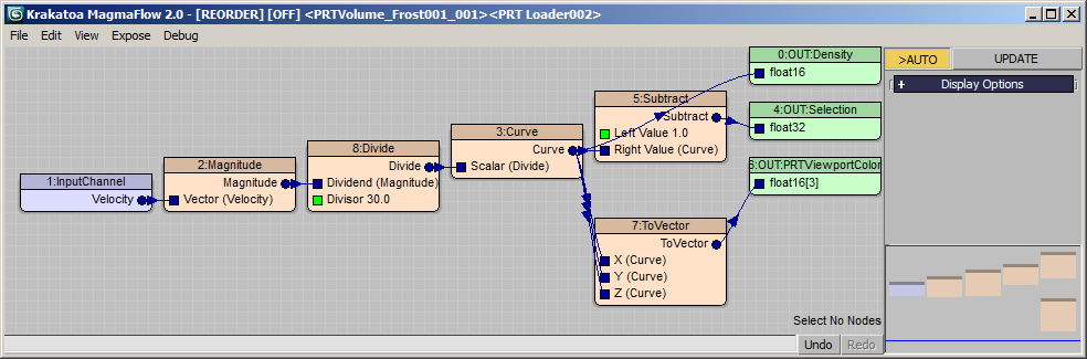
- Add another Magma modifier to the PRT Volume.
- Open the MagmaFlow Editor.
- Press Ctrl+O to create a new Output node, set it to Density channel.
- Press SHIFT+V to create a Velocity Input.
- Press V and M to create a Magnitude operator.
- Press / to create a Divide operator, enter 30.0 in the second slot’s default value.
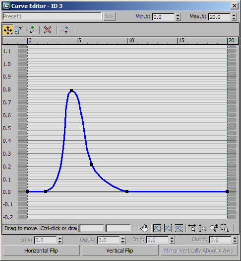
- Press F and U to create a Curve operator.
- Open the Curve operator’s floating editor
- Enter a Min.X and Max.X range from 0.0 to 20.0 in the top of the dialog.
- Tweak the curve to set the Density of particles in a small band to 1.0 while falling off to 0 in the rest of the range:
- Create two more Output nodes by pressing Ctrl+O
- Set the second to Selection and the third to PRTViewportColor
- Connect the Curve output to both new Output nodes.
- Select the wire to the second Output and press the - key to add a Subtract operator; press Ctrl+W to swap the first and second sockets. This produces a subtract from 1.0 setup.
- Select the wire to the third Output and press C for Convert and V for ToVector. Select both the Curve and the ToVector nodes by holding Ctrl and press SPACEBAR twice to connect all 3 components and produce a white color.
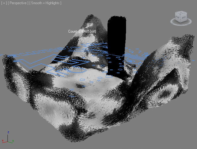
RESULT: We can now see which particles will be considered “foam” (white) and which will have low density and will disappear from the rendering (black). Using this grayscale preview, we could tweak the location of the foam particles by adjusting the Curve control and watching the viewport updates…
Rendering these particles will produce the following Krakatoa output:
Rendering As Krakatoa Atmospheric Effect
Krakatoa MX 2 adds the ability to render the particles as voxels in any renderer that supports the 3ds Max Environment effects, including Default Scanline, V-Ray, finalRender and Brazil r/s (excluding mental ray which requires rewriting of atmospheric shaders).
Obviously, this step cannot be peformed in Krakatoa 1.6.x and earlier.

We will use the Default Scanline renderer to render both the FROST mesh and the foam particles at once, including raytraced reflections and refractions.
- Select the PRT Volume and uncheck the “Subdivide Region” option - we won’t need that many particles for Atmospheric Rendering.
- On frame 200, enable the Auto Key mode of 3ds Max and enter 200 in the Random Seed of the PRT Volume. On frame 0, set the Random Seed to 0. Disable Auto Key. This will cause the PRT Volume to generate a different random pattern on each frame, producing a noise that is not static within the same volume from frame to frame.
- Unhide the FROST object and assign a Raytrace Material.
- Set the Diffuse Map to a Vertex Color Map (this will apply the Particle Colors calculated on the PRT Loader to the FROST mesh!)
- Set the Transparency to 212,212,212.
- Keep the IOR at 1.55
- Set the Specular color to white, Specular level to 50 and Glossiness to 40
- Add some Extra Lighting with a value of 72,89,99
- Optionally, create a Tube primitive around the pouring water portion of the particle system to represent the “hose” the particles are coming from.
- Open the Rendering > Environment dialog and add a Krakatoa Atmospheric effect.
- Press the Open GUI button.
- Press the “Add Particle Objects…” button and select the PRT Volume.
- Set Voxel Length to 1.0, Raymarch Step to 3.0
- Press the >Use button next to Light Density and enter 2.0/-1
- Set the Camera Density to 2.0/0
- Switch to Default Scanline Renderer and render frame 100
RESULT: Since the Voxel size (1.0) is smaller than the Spacing of the PRT Volume (2.0), some voxels will get particles and some will not. This produces a nice random noise pattern. The volumetric voxels are then refracted through the raytraced FROST mesh and are actually inside of the volume, giving the appearance of foam.

Using the Vorticity Channel
Assuming you have a BIN file sequence that contains a valid Vorticity channel, you can apply the same workflow outlined above and simply replace the Velocity channel with the Vorticity channel.
