Single Sided Meshing Of A Terrain Scan
Overview
- In the following tutorial, we will create a single sided mesh from a terrain scan.
- We will use a .LAZ file containing the aerial scan of the Serpent Mound park in Ohio, downloaded from http://www.liblas.org/samples/
Caching The LAZ File As SPRT
![[G]](../../_images/SQ_DOCS_GreenArrow_161.png) Create a Point Loader
Create a Point Loader 
Pick the downloaded .LAZ file.
- The Point Loader will look for a matching SPRT file, and if it does not find one, it will report a MISSING CACHE FILE in the Status field on red background:
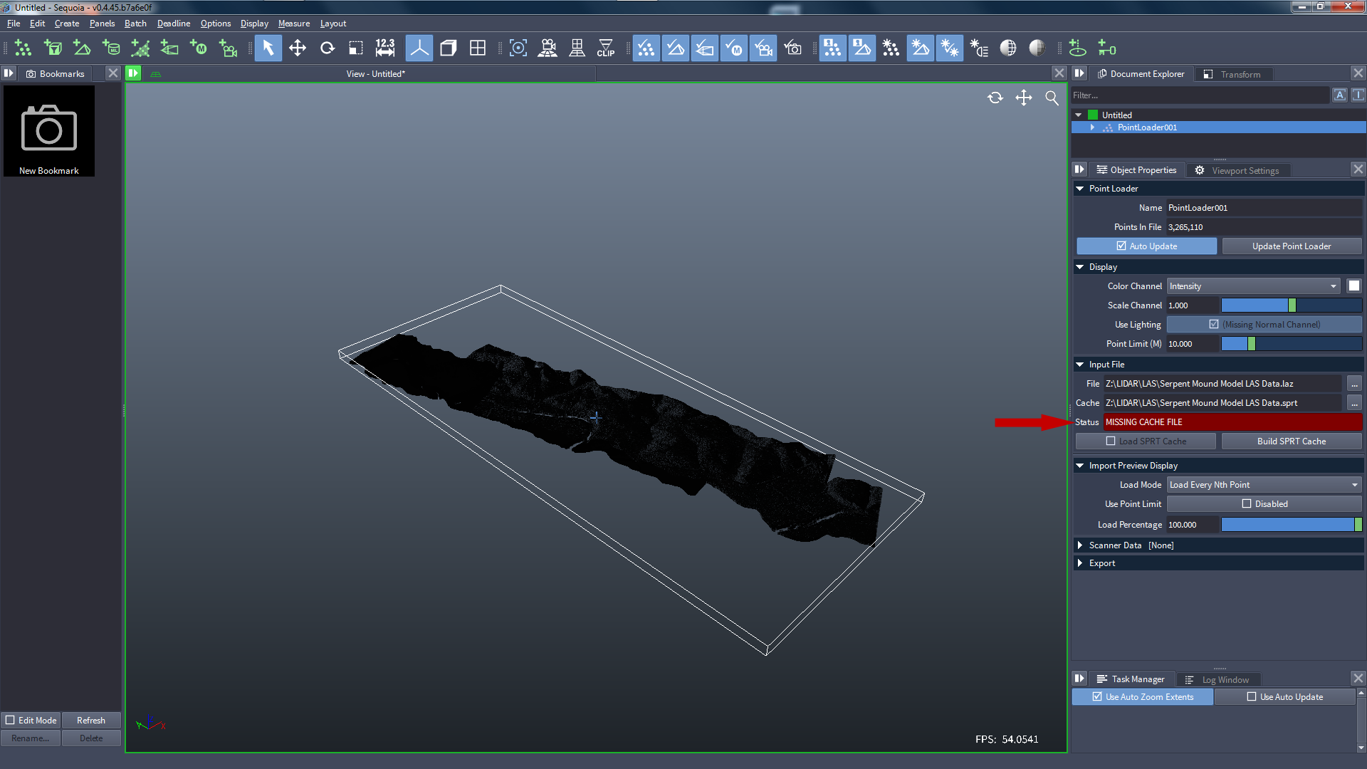
- The .LAZ file contains metadata describing the available channels.
- We can preview some of that data directly from the .LAZ file.
- For example, an Intensity channel is available and is displayed by default, however it is in a different scale, so it appears black.
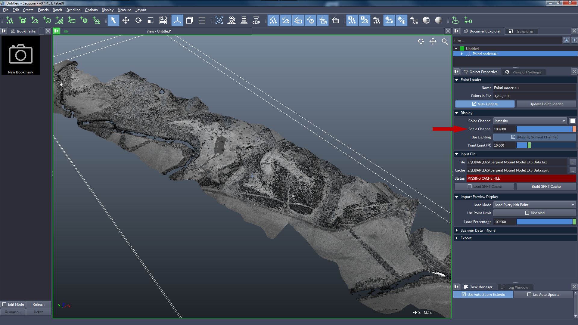
Change the Scale Channel value to 100.0 - this will multiply the Intensity and it will show up in the Viewport as a more useful grayscale value:
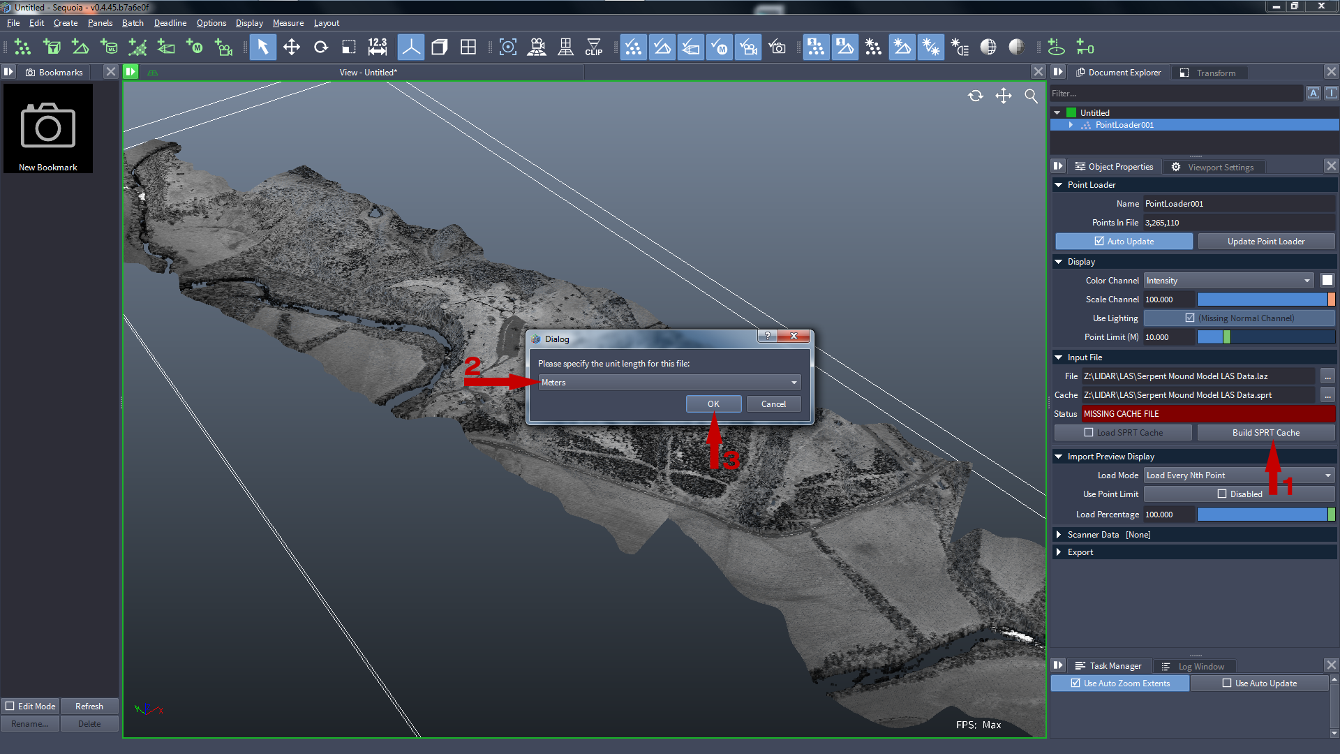
- The .LAZ file needs to be cached to .SPRT file
Pressing the Build SPRT Cache button [1].
- Since the .LAZ file does not contain any information about units, we will have to provide this information.
This particular file happens to be in Meters [2], so just confirm the suggestion by pressing OK [3]:
- The conversion will now be scheduled in the Task Manager.
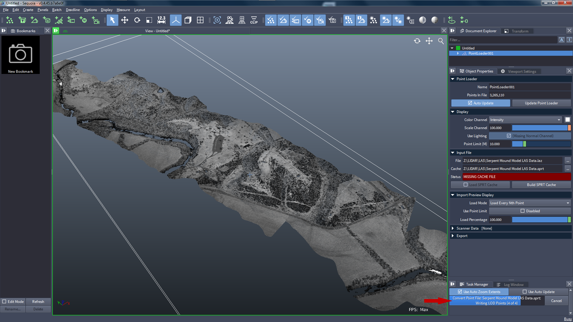
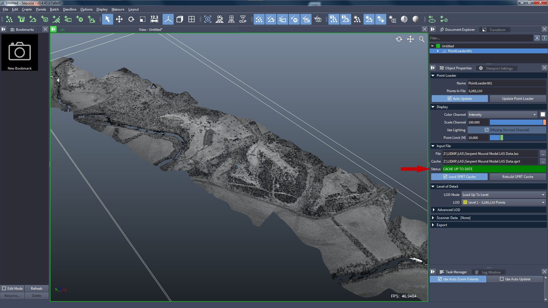
- After a few seconds, the SPRT cache will be ready and will be loaded automatically.
- The Status field will turn green and show CACHE UP TO DATE.
Generating Normals
- Now that we have the SPRT cache, let’s look into generating Normals.
![[R]](../../_images/SQ_DOCS_RedCircle_164.png) Note: The Point Normals Generation operator is not considered production-ready for general cases, but it tends to work well in the special case of terrain data where most normals point mainly up.
Note: The Point Normals Generation operator is not considered production-ready for general cases, but it tends to work well in the special case of terrain data where most normals point mainly up.
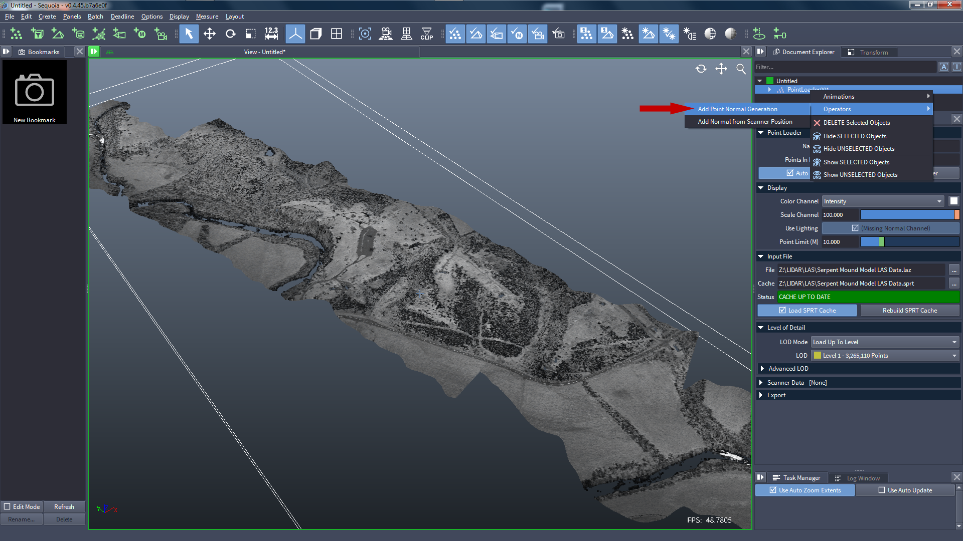
To add a Point Normals Generation operator, right-click the Point Loader and select from the Operators list:
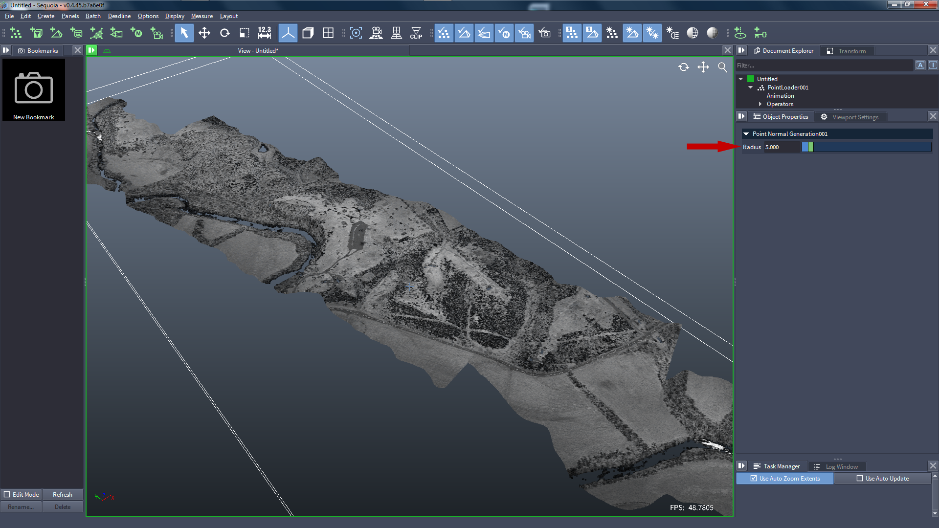
- The default Radius of 5.0 is a bit large for this data set.
Reduce the Radius value to 3.0 to speed things up:
![[B]](../../_images/SQ_DOCS_BlueRectangle_163.png) The original data set it located very far away from the World Origin, and some operations and display features become less precise at large offsets.
The original data set it located very far away from the World Origin, and some operations and display features become less precise at large offsets.
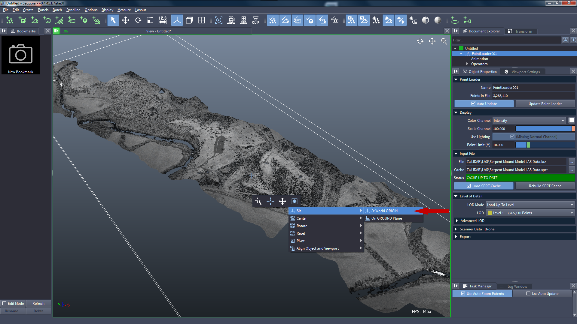
- In addition to generating Normals, let’s also move the point cloud to the World Origin.
Right-click the selected object and use the right-most menu to select Sit At World Origin”:
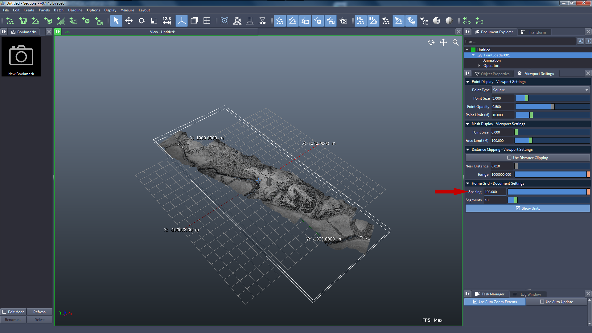
- Let’s resize the Home Grid to get a better idea of the size of the Serpent Mound park.
Enter 100.0 for the Home Grid Spacing
- With the default 10 subdivisions, we get a 2000 Meters long grid along each axis (from -1000m to 1000m).
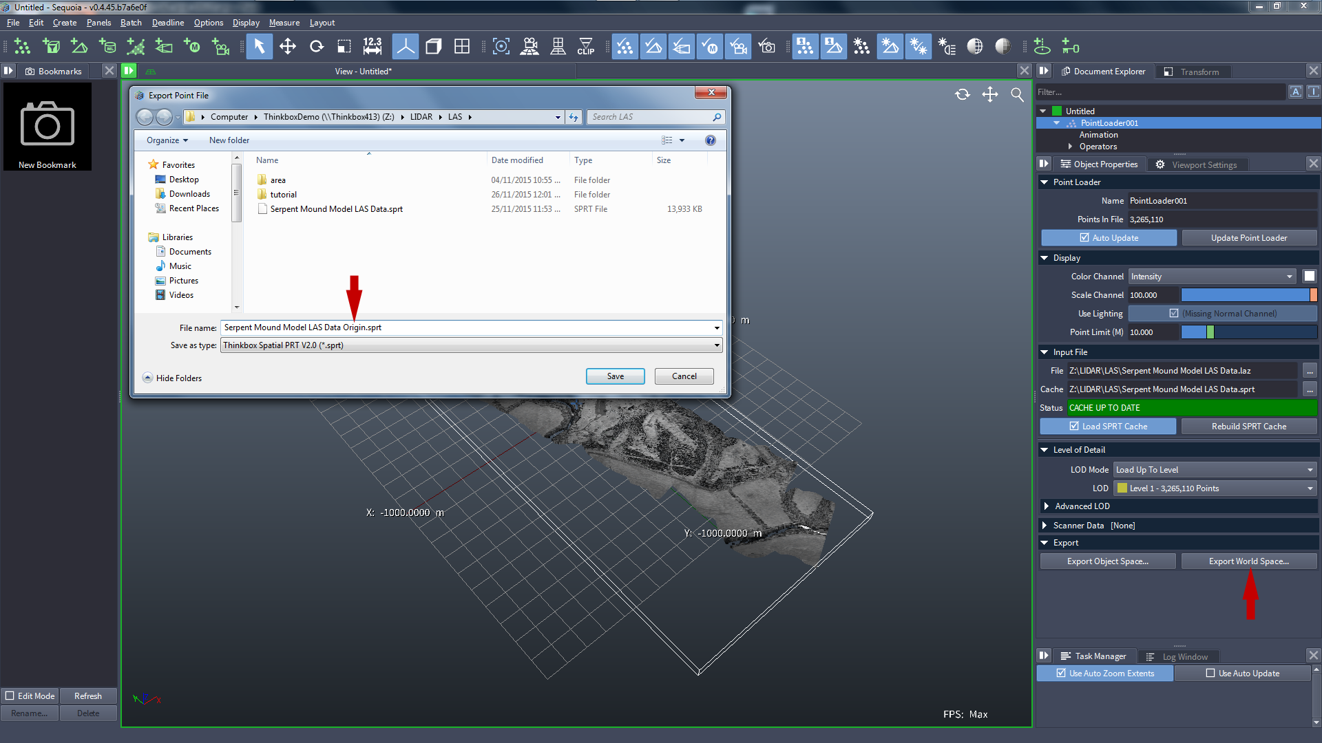
- We do not want to display the resulting Normals in the viewport, but we want to cache a new SPRT with the generated Normal channel already included.
Use the Export rollout’s Export In World Space button to bake both the translation to the World Origin and the new Normal channel to a new SPRT file with the suffix “Origin”.
Once the saving has finished, delete the original Point Loader.
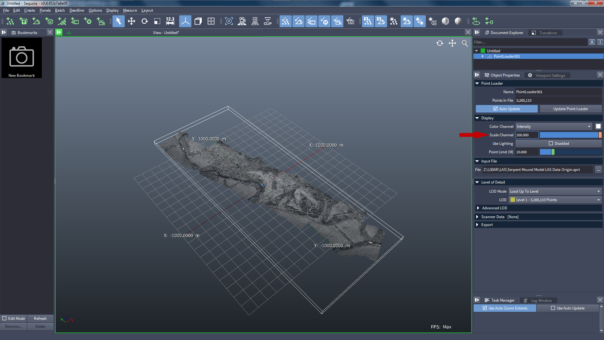
Create a new Point Loader and select the Origin SPRT file to read.
Be sure to scale the Intensity channel by 100.0 again.
- The file now contains valid Normals, so the points can participate in dynamic lighting.
Enable the Lighting in the Display rollout of the Point Loader.
By default, the Lighting of Points is disabled in the Viewports - check the Toggle Light Of Points... icon to enable:
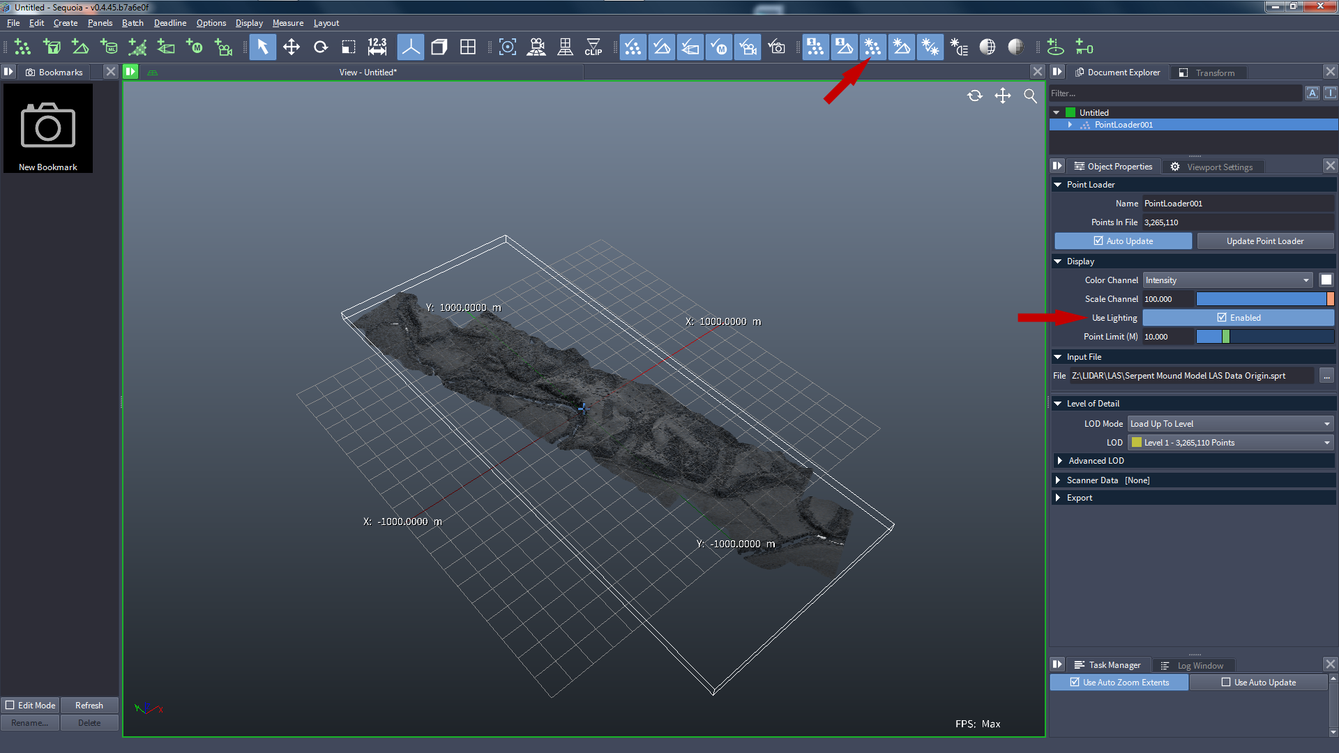
Instead of displaying the Intensity * Scale 100, switch to [User Color] value and set the Color Scale to 1.0 by right-clicking the slider and picking the DEFAULT value:
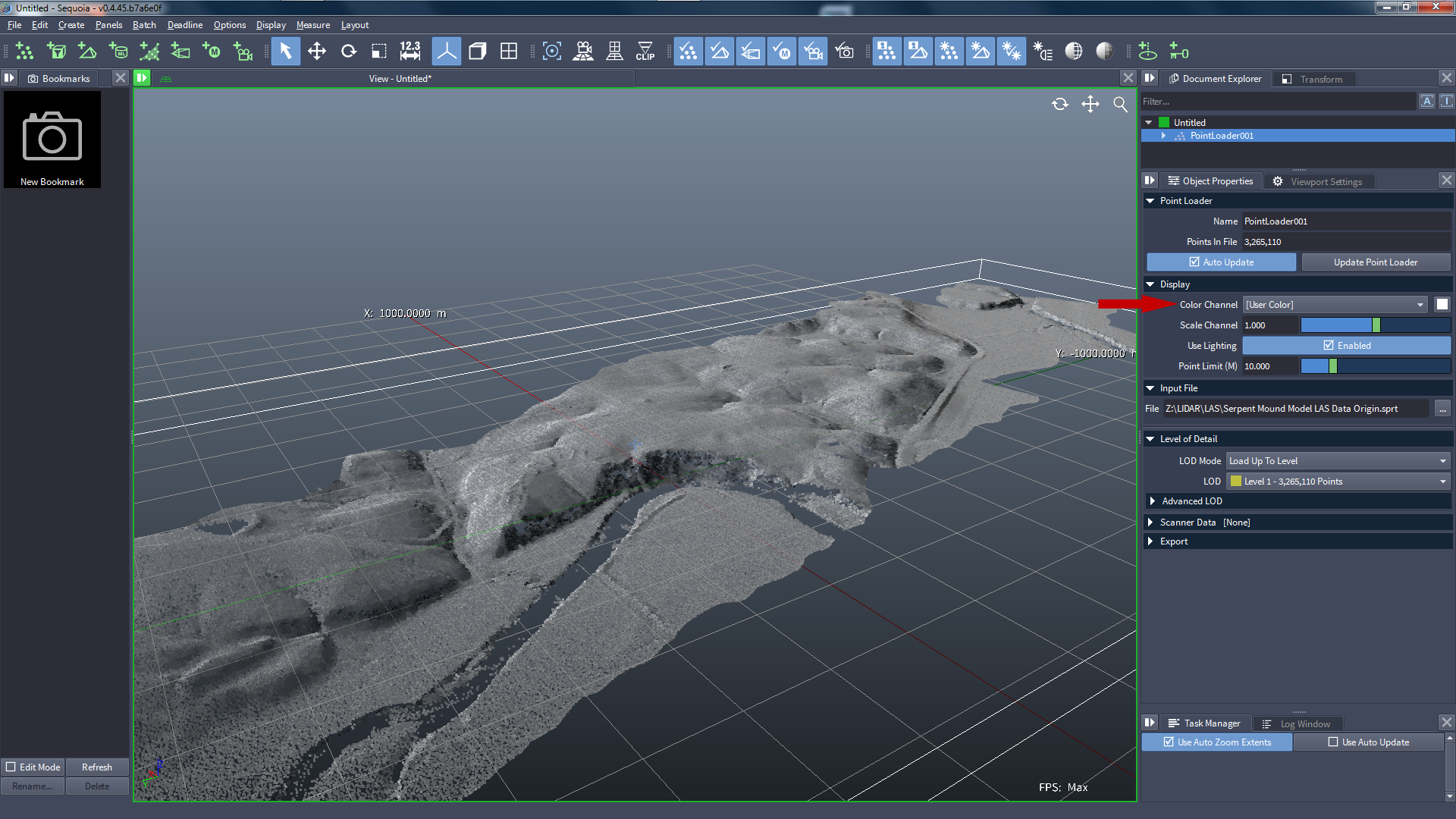
- As you can see, the points are shaded based on their new Normals!
Double-Sided Meshing
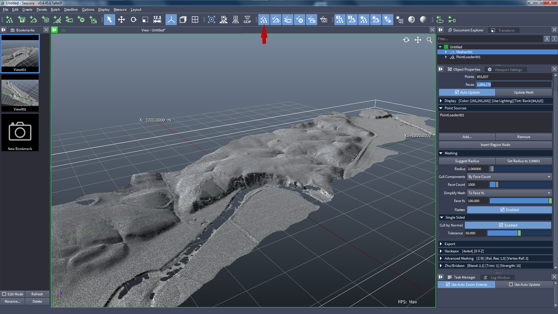
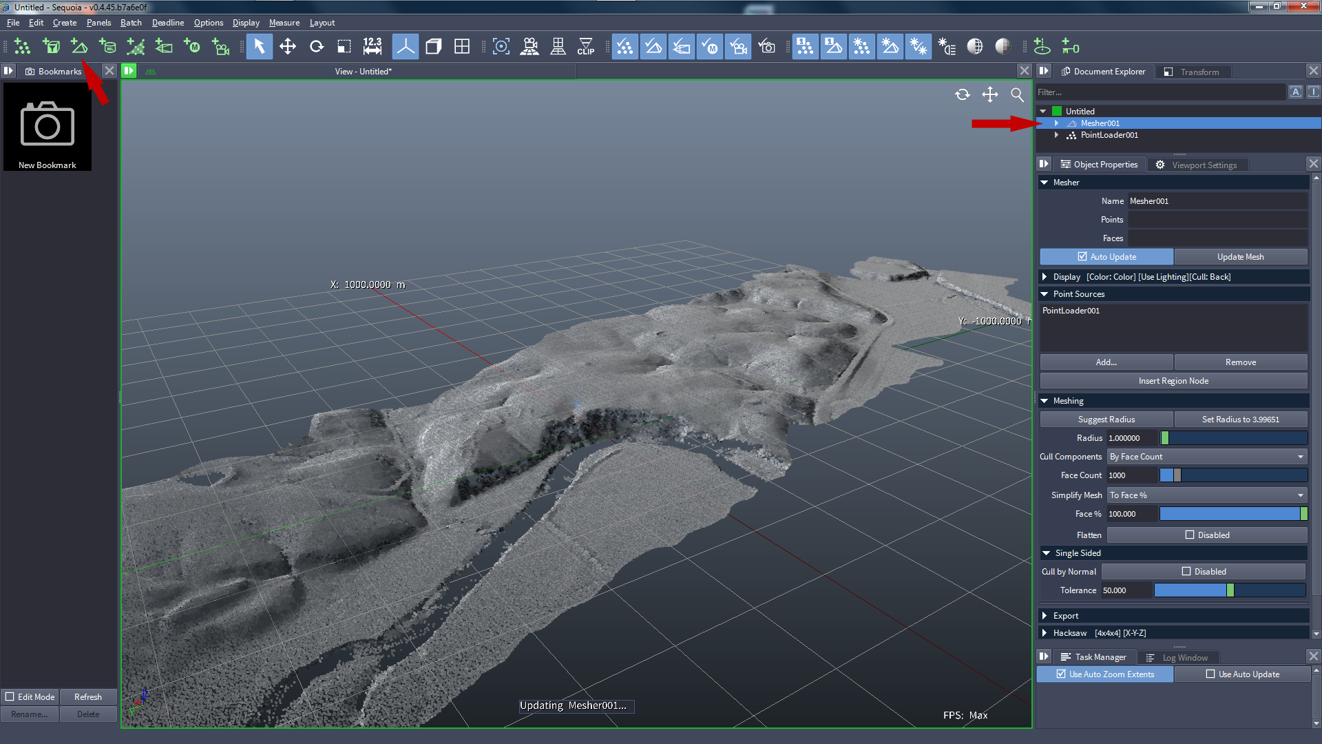
With the Point Loader still selected, create a new Mesher object by clicking on the 3rd icon from the left.
- The Mesher will be connected to the Point Loader automatically.
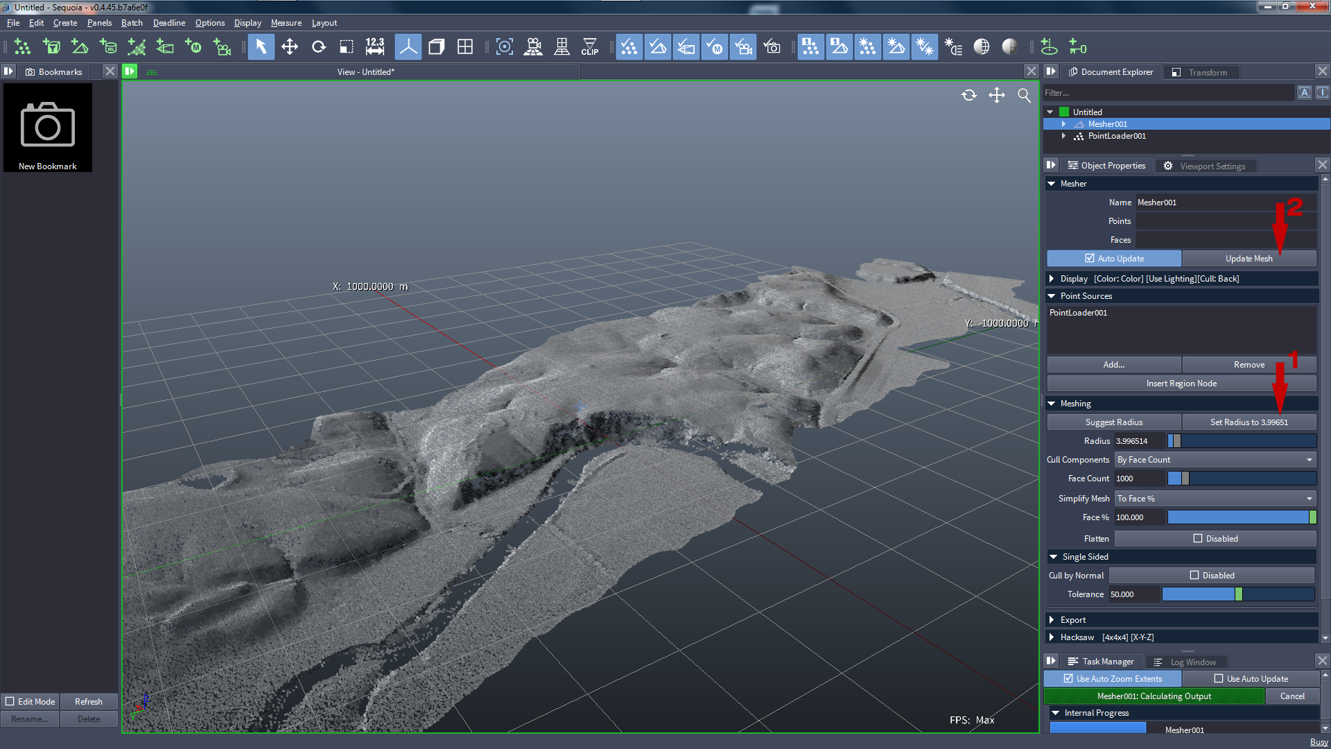
- It will suggest a possible Radius value based on the distance of the points in the cloud.
Accept the Suggested Radius by pressing the Set Radius to ... button [1].
Then press Update Mesh [2] to build the mesh:
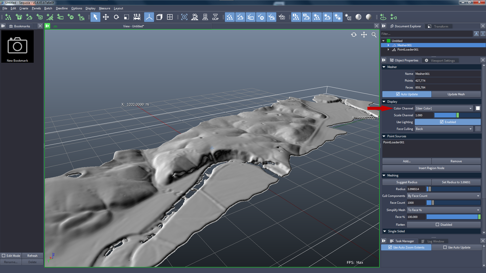
- The Mesher shows the Color channel by default, but the Point Loader did not have a Color channel, so the resulting Vertex Color channel is black.
Switch to [User Color] to show the mesh in White (or any other color):
- The Suggested Radius appears to be a bit too large (due to the nature of the data set which has quite a variable spacing).
Let’s halve it to about 2.0 units and press Update Mesh again:
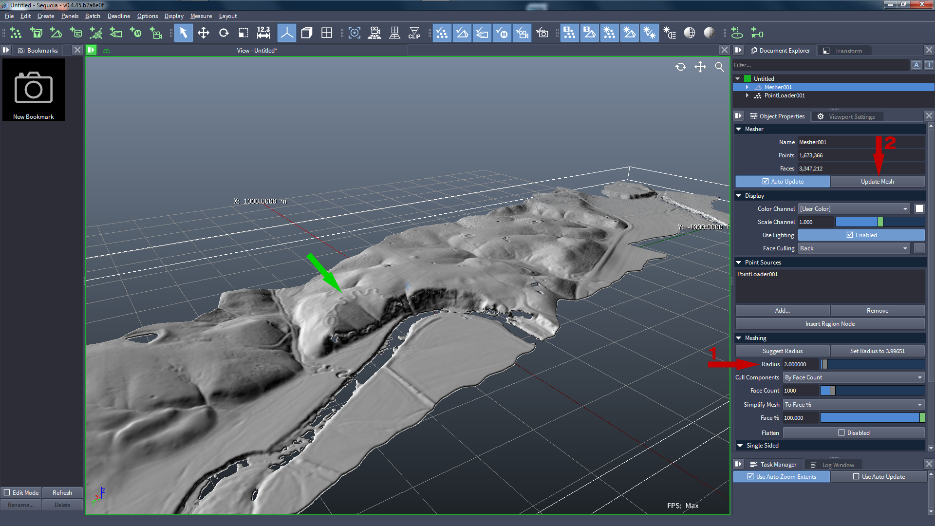
- This looks much better - the ancient Serpent shape can be recognized clearly on the terrain (green arrow).
Set a Bookmark to preserve the current view by clicking the New Bookmark icon in the Bookmarks panel.
Orbit the view to look at the underside of the mesh, and set another Bookmark to keep that view, too.
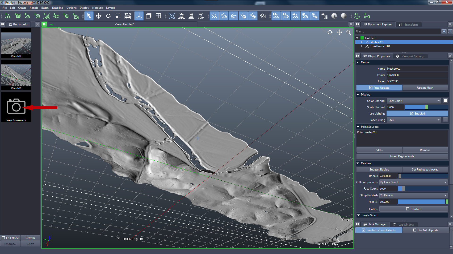
- The bottom looks pretty much the same as the top.
- In some cases, we want to remove this underside to reduce the number of polygons.
Culling Faces By Normal Similarity
When the Mesher finds a Normal channel in the Point Loader, it samples it into a channel called Mapping2.
Once such a mesh is created, the Cull By Normal option [1] can be enabled.
- This will enable a Cull Faces By Normal Similarity operator on the Mesher.
- It will compare the data in Mapping2 with the actual Normals generated by the Mesher, and will remove the back-facing polygons.
- Tweaking the value can remove more or less polygons depending on the angle between the two Normal vectors.
What would happen if the Point Loader did not contain a file with valid Normals?
In that case, an error would be displayed in the Task Manager, explainign that the Cull Faces By Normal Similarity requires a valid Normal channel in the point data.
Press the Update Mesh button [2] to remove the back faces - it should take just about a second to remove half the faces.
Disable the Points display in the Viewport [3] - we are only inrerested in the mesh now...
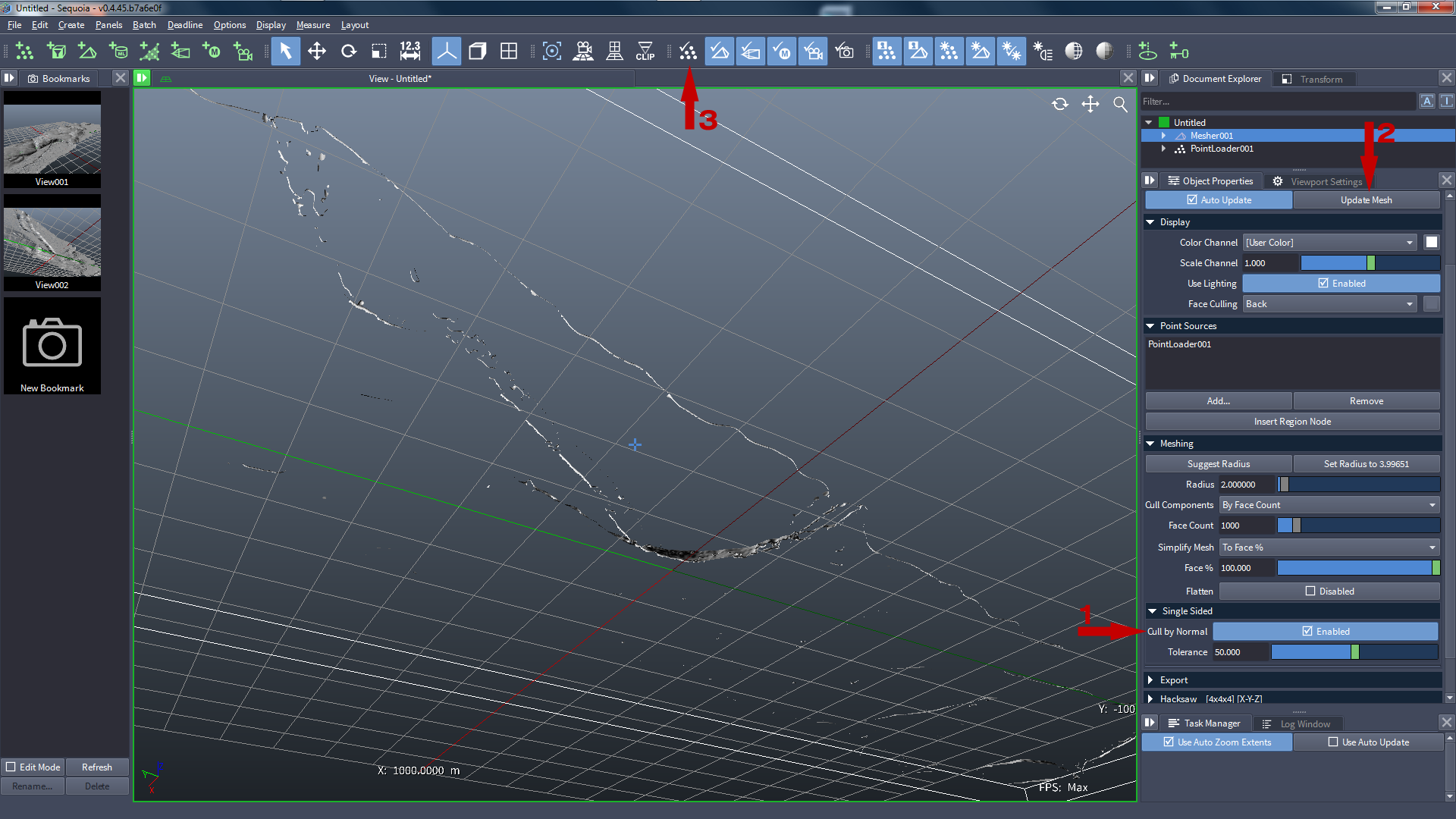
- As you can see above, the underside polygons are now gone because the Display defaults to backface culling.
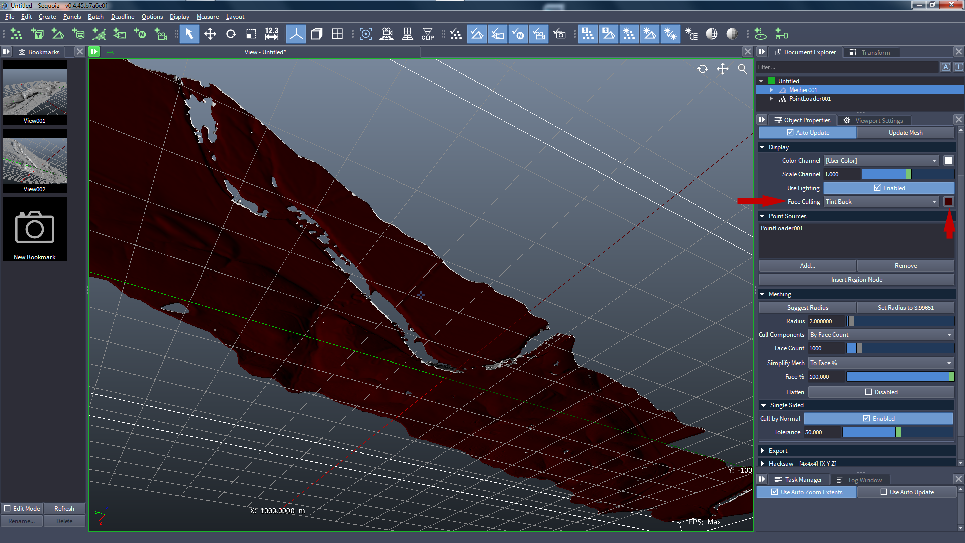
To visualize the two sides of the same polygons, switch the Display of the Mesher to “Tint Back”, and set the tint color to a shade of red.
- The result is that the front of the polygons will be shaded in white, and the backside will be shaded in red:
Conforming The Mesh To The Point Cloud
- At this point, the one side of the mesh still passes approximately 2 meters above the actual point cloud surface.
Check the Flatten option of the Mesher which enables a “Conform To Points” operator on the Mesher.
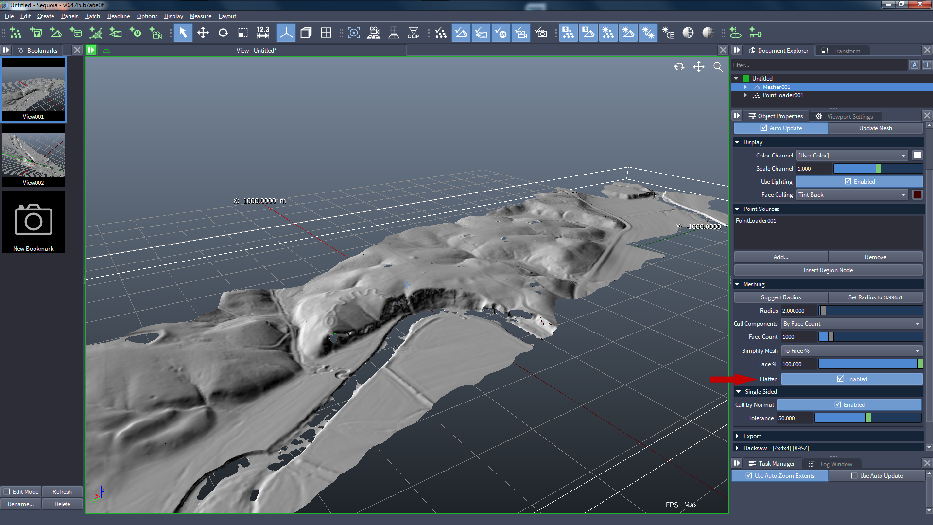
- As result, the single-sided mesh will be pushed down to the point cloud:
Enable the Point Display again to see that the Points and the Mesh surface are coincident now: