3ds Max Forces As Stoke MX Fields

Applicable to Stoke MX 2 and higher, Last Edited on June 6, 2014

Overview

The 3ds Max Force SpaceWarps are also Fields, and Stoke MX has always supported them as such when advecting particles. The main difference to Stoke Fields is that they are not used as Velocity Fields by 3ds Max itself, but as Acceleration Fields. In other words, they define the change in Velocity when applied to particles or other simulated objects, and will thus cause the Velocity to increase the longer the “Force” is applied.

Stoke MX generally accepts the value generated by a Force SpaceWarp as Velocity. This causes a particle to move with a speed that has the exact direction and magnitude provided by the SpaceWarp.

While it is possible to judge the nature of a 3ds Max Force SpaceWarp indirectly by the motion it produces in particles, the Stoke Field Magma object also provides a direct way to visualize the Field graphically in the viewports!

In the following tutorial, we will explore the shape of the various 3ds Max Force SpaceWarps using a Stoke Filed Magma object.

The illustrations will be taken from 3ds Max 2015 running Nitrous with Direct3D 9 which allows a very high number of samples to be drawn at reasonable speeds.

The Wind Force SpaceWarp

The Wind Force SpaceWarp has two component Fields - one is a procedural directional field (planar or radial), and the other is a Noise field.

• Start a new 3ds Max scene.
• Create a new Wind SpaceWarp from Create tab > Space Warps > Forces > Wind
• Place it at the World Origin 0,0,0
• Deselect the Wind object.
• Hold down the SHIFT key and use Stoke menu > “Create a Field MAGMA object…” to create a new default Stoke Field Magma object.
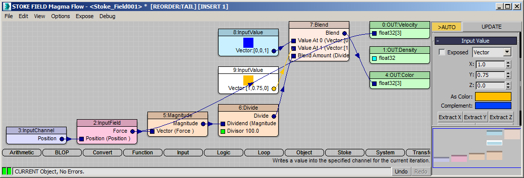
• Click the Open Magma Editor button.
• Select the Velocity Output node, then press I for Input, F for Field, and press ENTER to confirm.
• In the InputField node’s parameters, click on the Pick Field Source button and then pick the Wind from the scene.
• Drag a wire from the Position input socket and release over an empty area of the Editor to create and connect an InputChannel Position node.
• Press SHIFT+CTRL+C to create a new Color Output node.
• Connect the Force output of the InputField node to the Color Output node.
• Select the new wire and press V for Vector, then M for Magnitude.
• Press the / key on the Numeric Keypad to insert a Divide operator, then enter 100.0 as the default value of the second socket.
• Press F for Function, then B for Blend.
• Press CTRL+W and the SHIFT+CTRL+W to swap the first and second and then the second and third input sockets of the Blend.
• Press SHIFT+3 for a Vector InputValue with value of 0,0,1 (Blue).
• Press SHIFT+1 for a Vector InputValue with value of 1,0,0 (Red).
• Change the Y component to 0.75 to produce an Orange color instead of Red.

• Select the Stoke Field Magma object
• Change the Spacing to 1.0 - this will request over a million samples, but in 3ds Max 2015 the display is set to Reduce when 1 million samples are reached, so the Reduce: 1 display will show up in the viewport. In 3ds Max 2014 and 2013, only 100K samples are allowed by default, so the reduction will be higher.
• Under the Viewport Display rollout, press the Update Channels button.
• Change the Color drop-down list to Color.
• Change the Display drop-down list to Velocity.
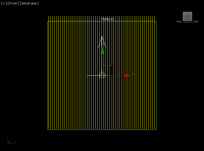
• Change the value next to the Norm.Length checkbox to 0.05 to scale down the line display.

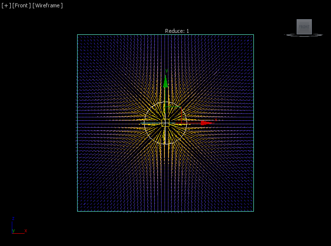
RESULT: The front viewport will now show the Forces of the default Planar Wind Force as vertical lines in yellow color:

Spherical Wind, No Decay

• Select the Wind SpaceWarp by name.
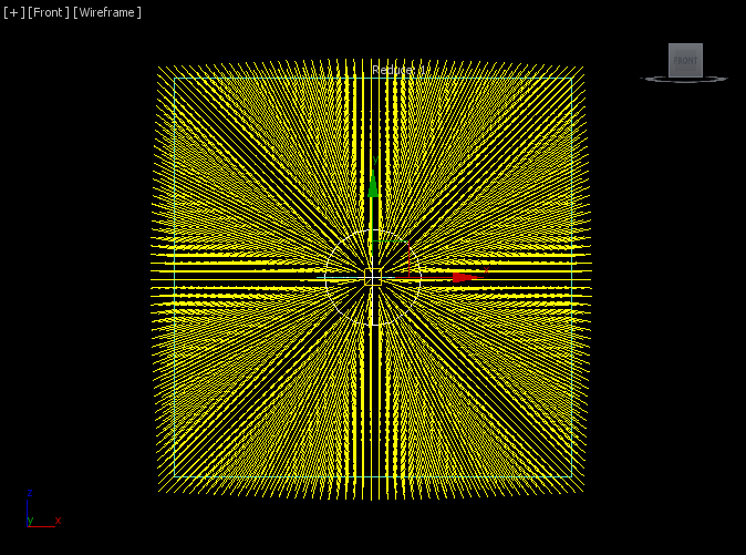
• Switch the Force radio buttons from Planar to Spherical.

RESULT: The vector field is now radial, pointing from the center out.

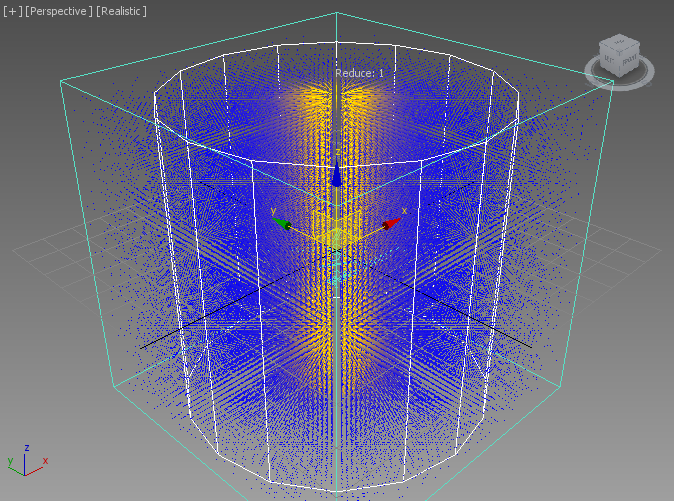
Spherical Wind, With Decay

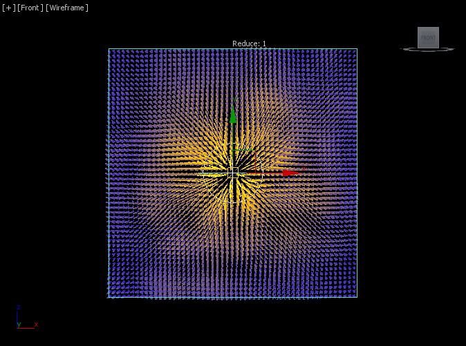
• Enter 0.025 for the Decay value.

RESULT: The Vector Magnitude (and thus the Color) now falls off from the center outwards.

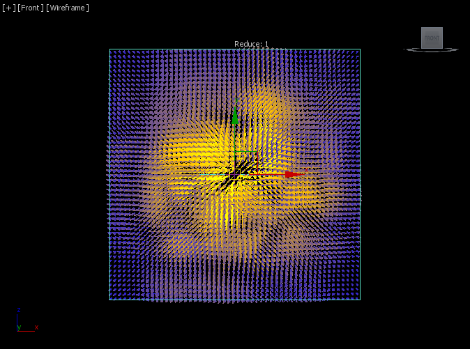
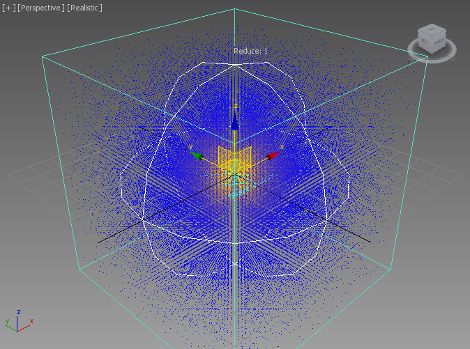
Noise Field Only (Turbulence)

• Set the Strenght value to 0.0 to turn it off
• Set Turbulence to 1.0.
• Set Frequency to 0.01.
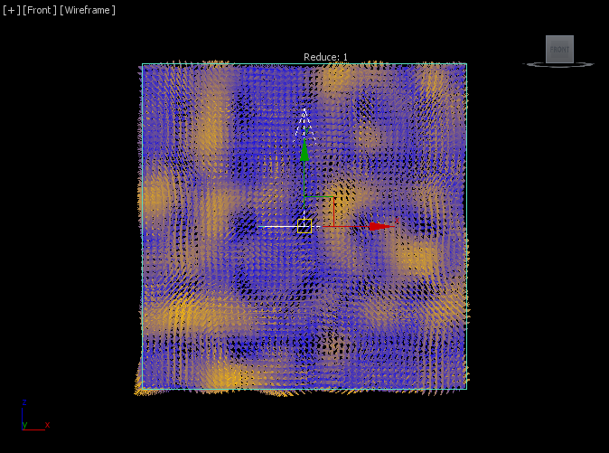
• Set Scale to 0.05.

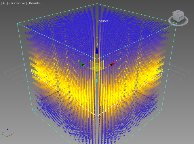
RESULT: This is the Noise Field in 3D space.

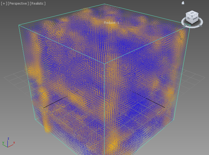
Here is the same in a Perspective view:

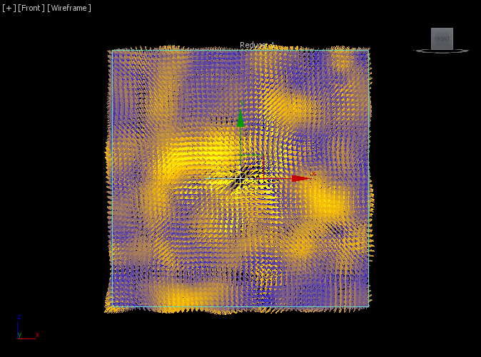
Mixing Radial Wind With Turbulence

• Enter 0.3 for Turbulence.
• Enter 1.0 for Strenght to enable it again.

RESULT: This is the combined Field of the Radial Wind and Turbulence Noise. The two are added together.

• Change the Turbulence to 1.0.

RESULT: The Noise Field is now too strong even where the Wind Strenght itself is nearly zero. This is because the Decay is only applied to the Strength but not to the Turbulence.

Combining Radial Wind Decay With Turbulence

To produce a combined field where both the Force Strength and the Wind Turbulence have the same Decay applied, we could

• SAVE the 3ds Max scene at this poimt
• Clone the Wind SpaceWarp as Copy
• Set the Turbulence of the first Wind to 0.0
• Set the Strength of the second Wind to 0.0
• Edit the Stoke Field Magma flow to load the second Wind, multiply its Force output by the Magnitude of the first Wind’s Force divided by 100.0, then add the two Forces together before outputting as Velocity and normalized Color.

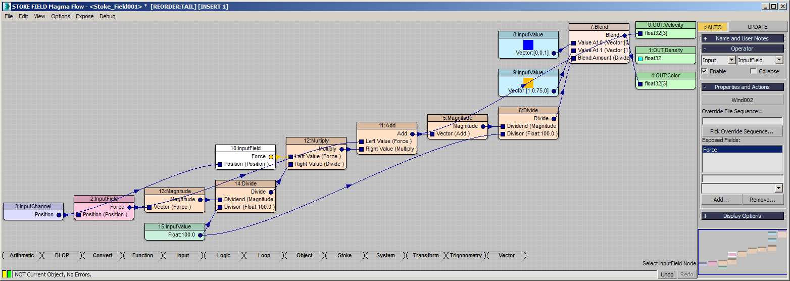
RESULT: The Turbulence field is now decaying together with the radial force:

So now we could pick the Stoke Field Magma as our Force source instead of the actual Wind SpaceWarps and use it to drive Stoke particles or PFlow Particles. Or we could turn it back to a Force by creating a Stoke Field Force object and picking the Stoke Field Magma as the source and Velocity as the channel.

In other words, we can take existing 3ds Max Forces, reprocess them via a Magma flow, and create new, previously not existing Forces that can be used in the same places inside of 3ds Max!

The Displace Force SpaceWarp

The Displace Force can be used both as a deformer to shift vertices of a mesh, and as a particle force field. Obviously, Stoke MX 2.0 can use it as a Field to affect particles, but the Genome modifier which is also part of the Stoke MX 2.0 package could read it as a source of particle deformations.

• SAVE the 3ds Max scene from the previous step under a new name.
• RELOAD the previous 3ds Max scene with the single Wind field.
• Select and delete the Wind object - the Stoke Field Magma will become invalid and the samples will disappear from the viewport.
• Create a Displace SpaceWarp at the World Origin [0,0,0]
• Set the Length and Width properties to 50.0.
• Pick the Displace as the source in the Stoke Field Magma’s InputField node.
• Enter 10.0 for Strength - a field of vertical vectors with yellow color like with the Planar Wind will apepar.
• Set Decay to 4.0.

RESULT: The Field will decay relative to the Plane.

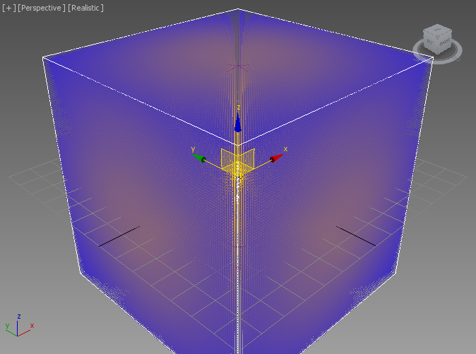
Cylindrical Displace

• Change the Map mode to Cylindrical
• Set Height to 100.0.

RESULT: The Decay is now radial perpendicular to the vetical axis of the Cylinder

Spherical Displace

• Change the Map mode to Spherical
• Set Height to 50.0.

RESULT: The Decay is now radial like in the Radial Wind mode. Changing the Decay to 1.0 would produce a very simular Field to the Radial Wind with Decay of 0.025 we created previously.

Tweaking The Viewport Sample Limits

As mentioned already, 3ds Max 2015 allows a lot more samples to be drawn in the viewports at high speeds. But right now, with a Spacing of 1.0 and a Grid slightly larger than 100 units in each direction, we are requesting more than 1 million samples, and a Reducation of 1.0 kicks in automatically to ensure we don’t draw more than 1 million samples.

This limit is actually customizable, but is only exposed to MAXScript. When Stoke MX 2.0 is started, it checks the version of 3ds Max and Nitrous that is being used, and sets the viewport limit for an individual Field object to be 100,000 for 3ds Max 2014 and earlier, and 1,000,000 for 3ds Max 2015.

The MAXScript Interface property responsible for this limit is called StokeGlobalInterface.MaxMarkerCount

In this example, all screenshots were made using 3ds Max 2015 and Nitrous Direct3D 9 drivers. We can allow more than 1 million samples to be drawn by evaluating in the MAXScript Listener

StokeGlobalInterface.MaxMarkerCount = 10000000

This will allow up to 10 million samples to be drawn for a single Stoke Field object!

• Change the Decay from 4.0 to 1.0.
• Select the Stoke Field Magma object and toggle the On checkbox under Viewport Display off and on again.

RESULT: All 1,191,016 samples will be drawn in the viewports.

We can still force a Reduction of 1 by entering 1 in the Reduce value field under the Viewport Display rollout.

Displace Mapping

The Displace SpaceWarp also allows a bitmap or procedural maps to be used to modulate the Displacement Strength in the specified mapping space.

• Switch to Planar Map again.
• Change the Decay back to 4.0.
• Click the Map button and pick a default Checker map.

RESULT: The Strength will be 0 in the Black squares of the Checker map, and will behave as before in the White squares.

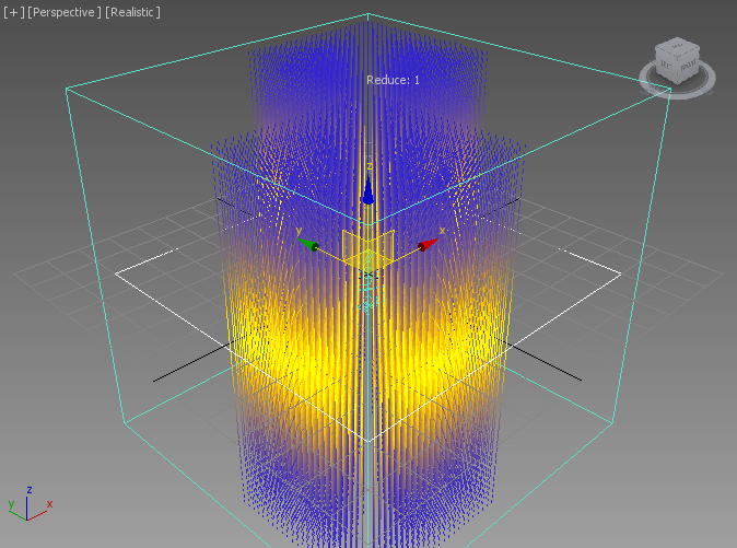
• Replace the 2D Checker map with a 3D Cellular Map
• Change the Decay to 2.0 to see the field better

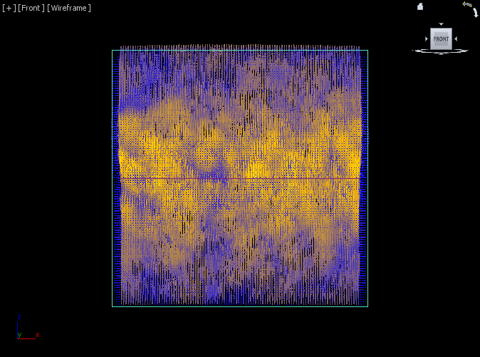
RESULT: The forces are still vertical and parallel to the plane of the Displace SpaceWarp, but their Magnitude is affected by the color of the Cellular map:

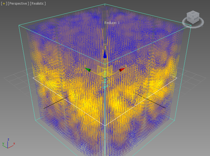
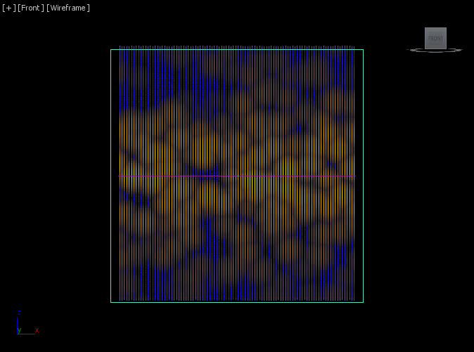
• Change the Reduce from 1 to 0 to see all samples.
• Look in the Front viewport.

RESULT: We can see the 3D Cellular Map distributed throughout the volume of the grid, modulating the Strength of the Displacement effect while preserving the vertical orientation of the field.

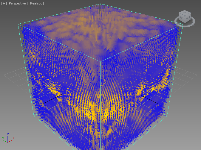
Here is what it looks like in the Perspective Viewport:

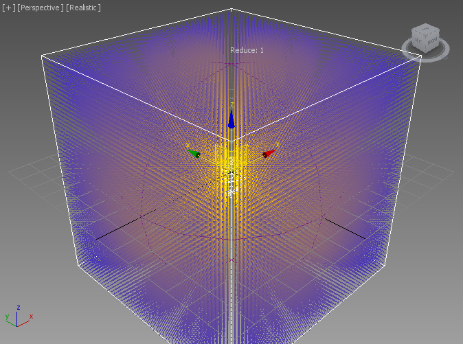
Creating A Simple Fluid - Removing Divergence

As we already know, we can use the SimpleFluid node in Magma to remove the Divergence from the Field and ensure that the amount of fluid entering every point in space is equal to the amount leaving it.

• Select the InputField operator in the Magma flow.
• Press S for Stoke category, then F for SimpeFluid - a new node will be inserted into the flow.
• Drag a wire from the Position input socket of the SimpleFluid and release over an empty area of the Editor - it will be automatically connected to the existing Position node.

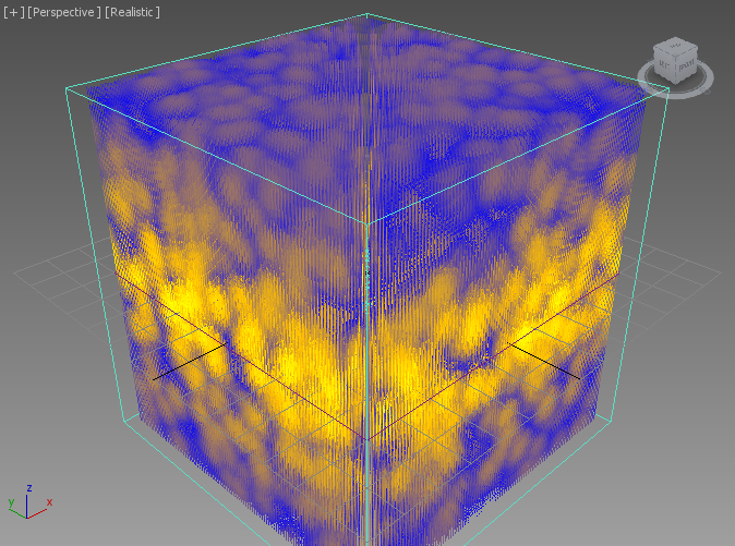
RESULT: After a short calculation, the viewport will show a modified, Divergence-Free Field.

And here it is in the Perspective Viewport: